 aws-analyzer · s3.py
Explore your S3 data from a SageMaker notebook
Install it in your notebook and get readable reports on your buckets: what's in them, what they cost, who can read them, and what's inside the files, without leaving Jupyter.
- One install, boto3 only
- Read-only: never changes your data
- Works on billion-object buckets
- Plain text outside Jupyter
Every example uses a bucket called acme-ml-data; use your own bucket names. The screenshots are real output from the tool, run against a demo bucket with synthetic data.
Set up in SageMaker
-
Install the package, in a notebook cell:
%pip install aws-analyzerNo internet in the notebook (VPC-only mode)? On a computer that has internet, download the package and copy it to a bucket the notebook can read (
pip download aws-analyzer --no-deps -d wheels, thenaws s3 cp --recursive wheels/ s3://acme-ml-data/tools/wheels/), and install it from there:!aws s3 cp --recursive s3://acme-ml-data/tools/wheels/ wheels/ %pip install --no-index --find-links wheels aws-analyzer -
Import it and create the view. It uses the notebook's IAM execution role, so there's nothing to configure.
from aws_analyzer import S3View ui = S3View() # uses the notebook's IAM role ui.help() # every command, grouped by task; ui.help("summary") shows one in full -
Optional: another AWS profile or region, plain-text output, or longer tables:
from aws_analyzer import S3Analyzer, S3View

ui = S3View(S3Analyzer(profile="dev", region="eu-west-1"))
ui = S3View(mode="text")          # plain text, e.g. in a terminal or a script
ui = S3View(max_rows=0)           # show every row of long tables (default: 50)
ui = S3View(progress="plain")     # a plain progress line instead of tqdm bars ("off" for none)
ui = S3View(downloads="~/scratch/s3")   # where downloads go (default: s3-downloads, next to the notebook)
Only boto3 is required. pandas, pyarrow and numpy (all preinstalled on SageMaker) are used for tables. A few file types need an extra package; the preview tells you which one when it's missing:
%pip install openpyxl pypdf pypdfium2 pillow zstandard python-snappy # Excel, PDF text and pages, .zst before Python 3.14, snappy Avro
Commands that take a while show a tqdm progress bar with the time left, when tqdm is installed (it usually is on SageMaker; ipywidgets makes it a notebook widget). Without it you get a plain line with the same numbers.
Five-minute tour
The commands you'll use most. Each one prints a report under the cell; none of them change anything.
ui.overview()                                        # every bucket: size, monthly cost, warnings
ui.bucket_info("acme-ml-data")                       # settings, policy, risks, size by storage class
ui.summary("s3://acme-ml-data/curated/")             # what's in a folder, and what it costs
ui.find("s3://acme-ml-data/", extensions="parquet", min_size="100MB")
ui.preview("s3://acme-ml-data/curated/features/churn/train.parquet")
df = ui.core.read_df("s3://acme-ml-data/curated/features/churn/train.parquet")   # a pandas DataFrame
Reading a report. Every report puts the answer first: cards with the numbers that matter (a card turns amber or red when a finding is about it), then the findings, warnings first, each a bold headline with why it matters and what to do underneath. The tables of detail come after, with status cells such as FAILED in colour. Click a column's header to sort by it (again for the other way, a third time for the original order), pick a value in a column's Filter to see only those rows (a storage class, a region, a bucket), and untick columns under Columns to focus on the ones you need. Keys start with an icon for the kind of file (📊 a table, 📕 a PDF, 🧠 a model, 📁 a folder) and keep the file name in view: the folder is dimmed and shortened from the left, and the whole key shows when you hover over it. It's all plain HTML and CSS, so it still works when you reopen the notebook. At the bottom is a Next row of two or three commands with the arguments filled in from this report, such as tree('s3://acme-ml-data/curated/'). One click on a command anywhere in a report, or on a code block, selects all of it, ready to copy. ui.help() lists every command by task; ui.help("summary") shows one in full.
Anywhere a location is expected you can write s3://bucket/prefix or just bucket/prefix. Sizes accept 1024, "10MB" or "1.5GB". Times accept a datetime, "2025-05-01", or an age such as "7d", "12h" or "2w" (meaning that long ago).
Click through folders
Rather click than type paths? s3_explorer.py turns a cell into a file explorer for S3: your buckets and folders on the left, and on the right whatever you click, read by the same preview as the reports here. Put it next to s3.py and run:
from aws_analyzer import S3Explorer

S3Explorer("s3://acme-ml-data/curated/")   # or S3Explorer() to start from your buckets
The S3 explorer guide covers setting it up, every button, reading a PDF page by page, zipping a folder, and driving it from code.
Your buckets
Every bucket at a glance
overview() checks every bucket in parallel: size and object count (from CloudWatch, so it's instant even for huge buckets), estimated monthly cost, versioning, encryption, public access, lifecycle rules, and a list of warnings.
ui.buckets()                      # just names, regions and creation dates (fast)
ui.overview()                     # every bucket in one table
ui.overview("sagemaker-*")        # only buckets whose name matches
ui.overview(metrics=False)        # skip CloudWatch: faster, but no sizes or costs
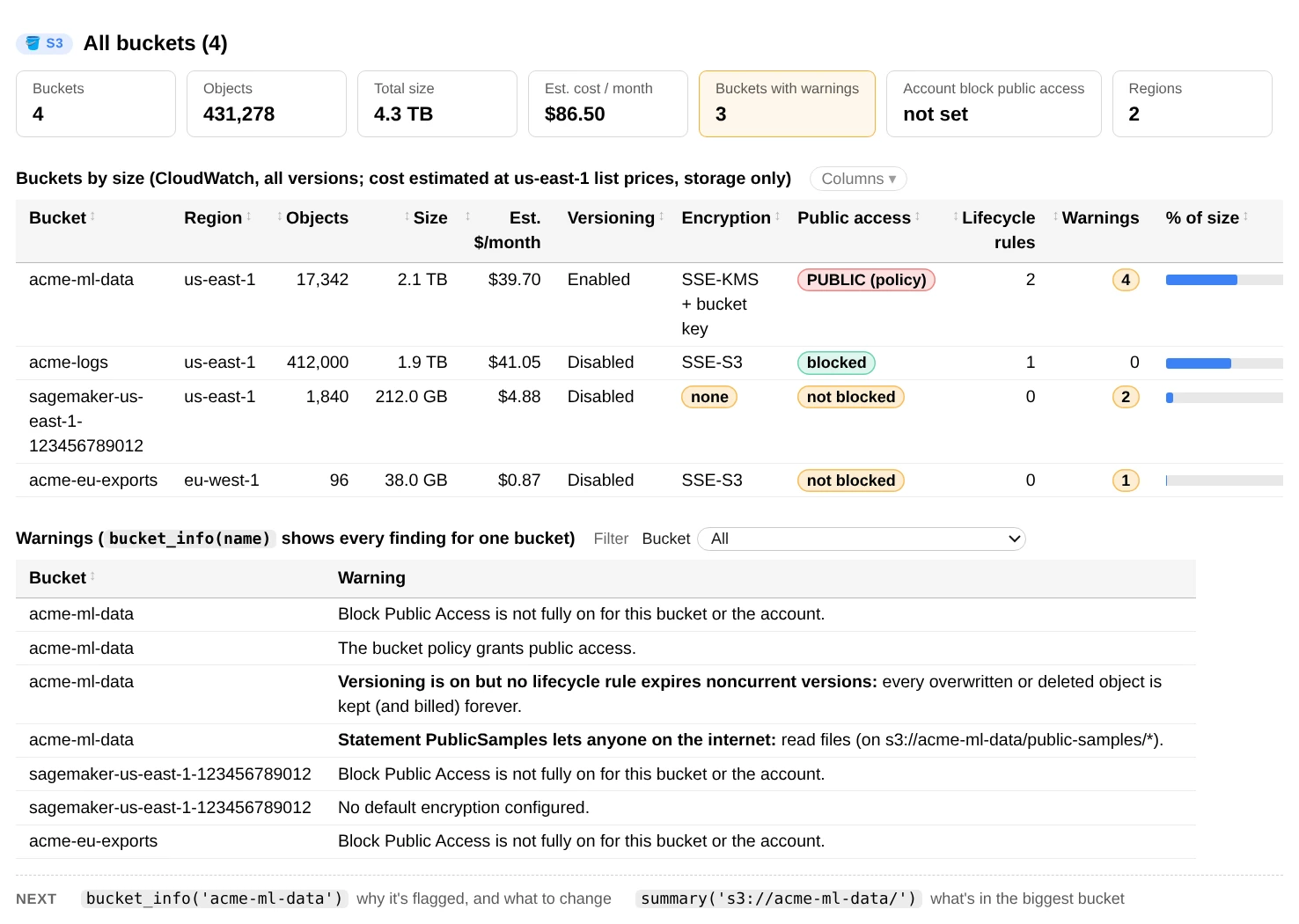
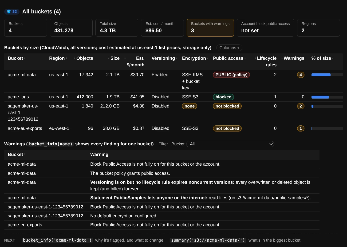
ui.overview(): sizes and costs cover all versions, from CloudWatch's daily storage metrics.
One bucket in detail
bucket_info() shows the bucket's settings and flags anything risky or wasteful: Block Public Access off, no default encryption, versioning without a rule that cleans up old versions, and so on. It also explains the lifecycle rules and the bucket policy in plain English, and prices each storage type.
ui.bucket_info("acme-ml-data")
ui.bucket_info("s3://acme-ml-data/any/path")   # a full S3 path works too
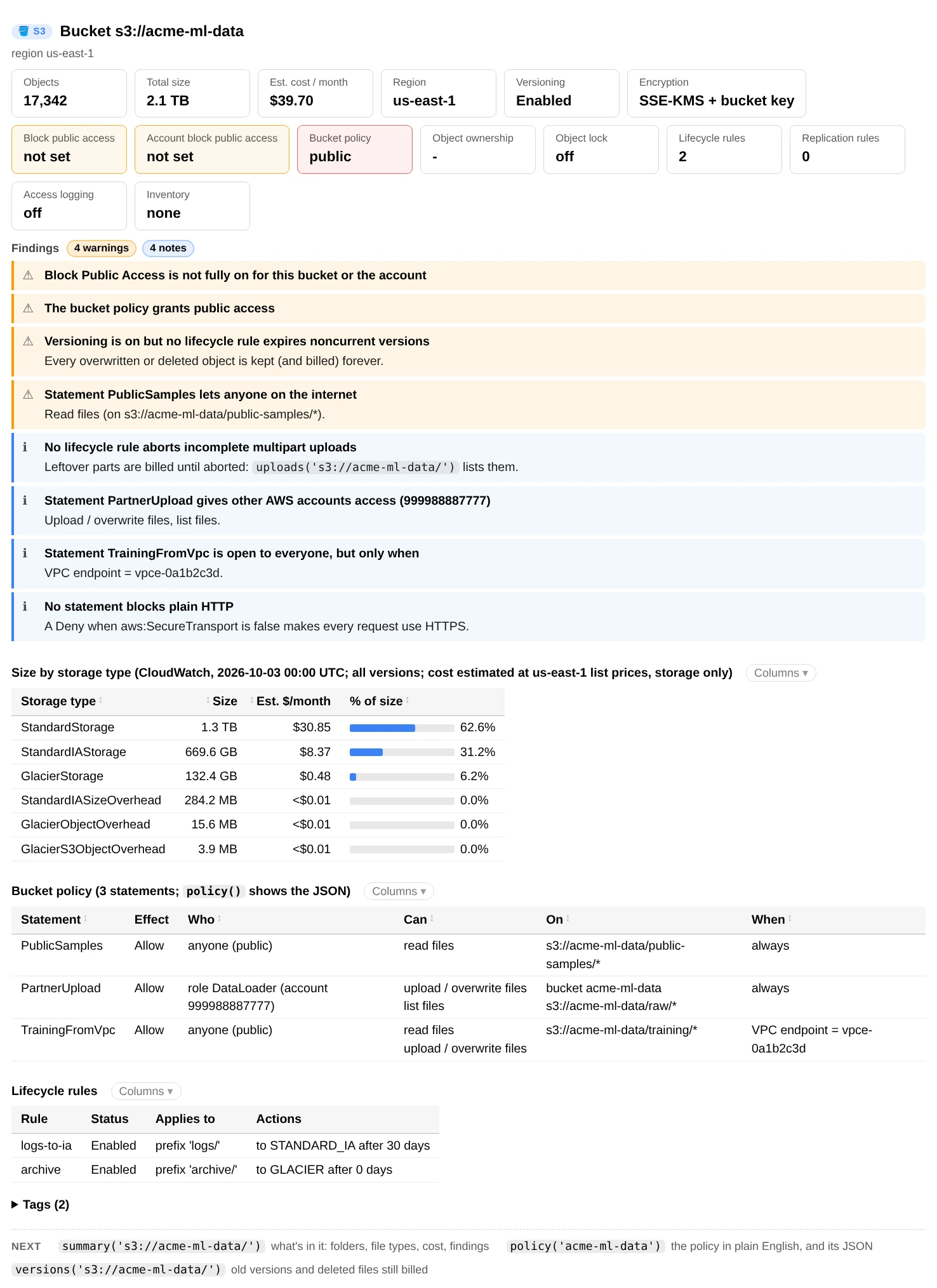
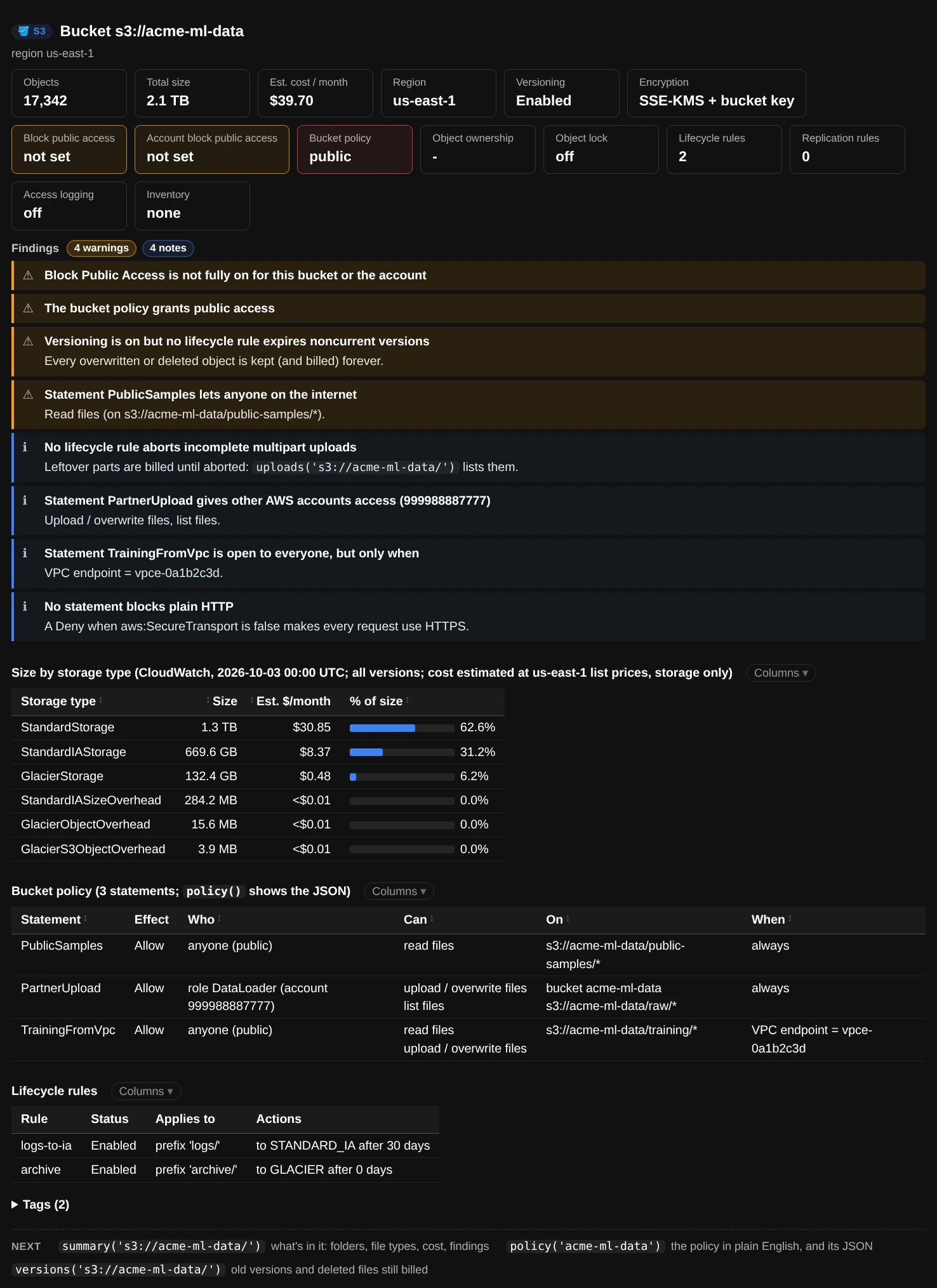
ui.bucket_info("acme-ml-data")
Who can access a bucket
policy() turns the bucket policy into a table of who can do what, on which files, and under which conditions. It flags statements open to the whole internet, access from other AWS accounts, and whether plain HTTP is allowed. The raw JSON is shown underneath.
ui.policy("acme-ml-data")
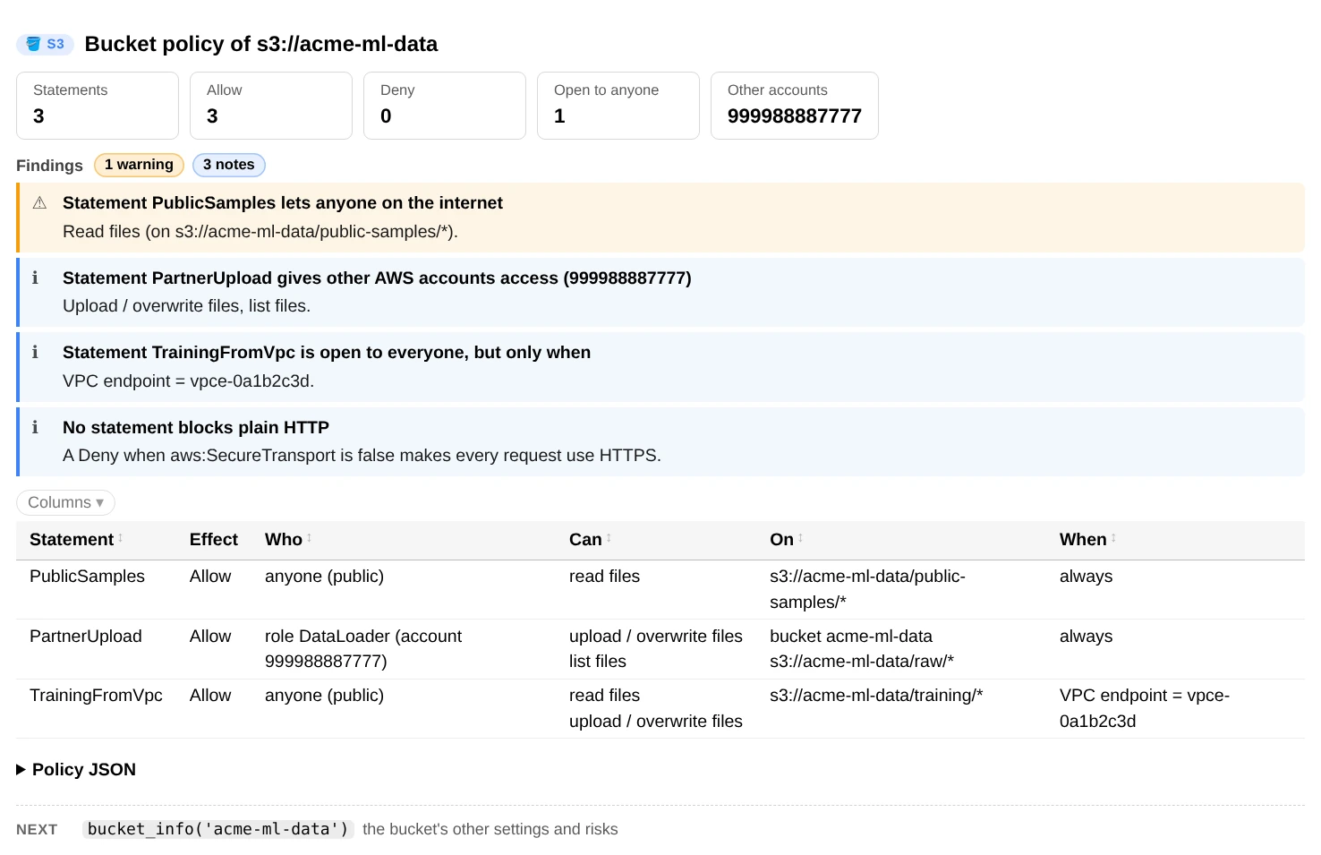
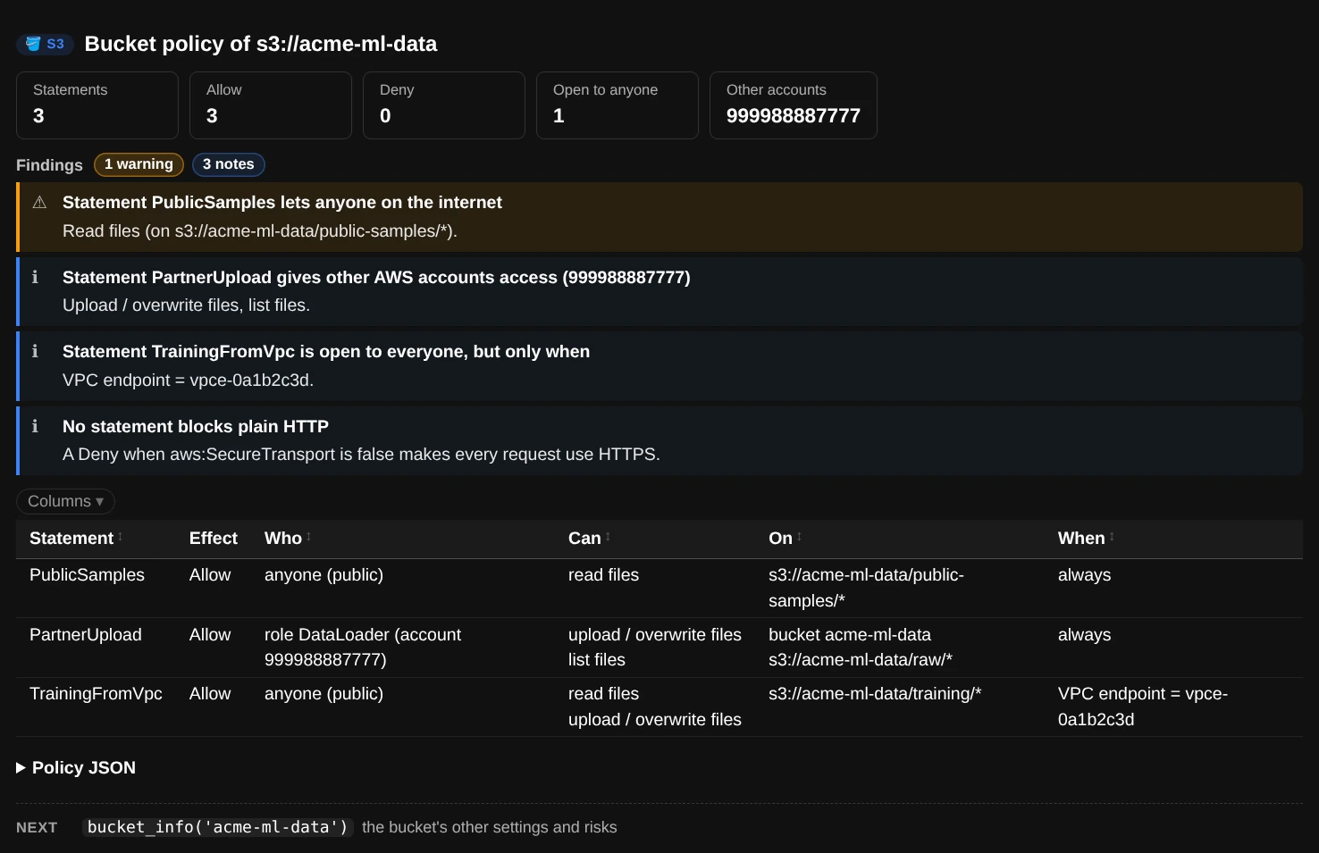
ui.policy("acme-ml-data")
Browse and search
Folders
ui.ls("s3://acme-ml-data/")                        # one level, like `aws s3 ls` (fast anywhere)
ui.ls("s3://acme-ml-data/training")                # 'training' is read as the folder 'training/'
ui.ls("s3://acme-ml-data/docs/", details=True)     # + what's inside each file: pages, rows, picture sizes
ui.tree("s3://acme-ml-data/curated/", depth=3)     # size and object count at every level, with the files
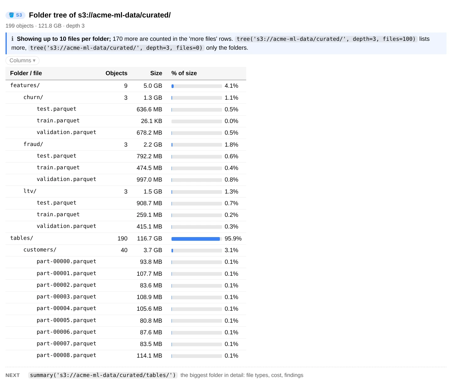
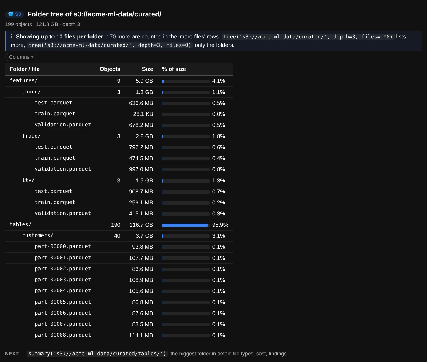
ui.tree("s3://acme-ml-data/curated/", depth=3)
Find files
Combine any filters; a file has to match all of them.
ui.find("s3://acme-ml-data/training/", pattern="*.tar.gz", min_size="4GB", modified_after="90d")
ui.find("s3://acme-ml-data/raw/", regex=r"dt=2025-0[1-3]-\d\d/", extensions=["json", "csv"])
ui.find("s3://acme-ml-data/archive/", storage_classes="GLACIER", limit=None)   # no cap on matches
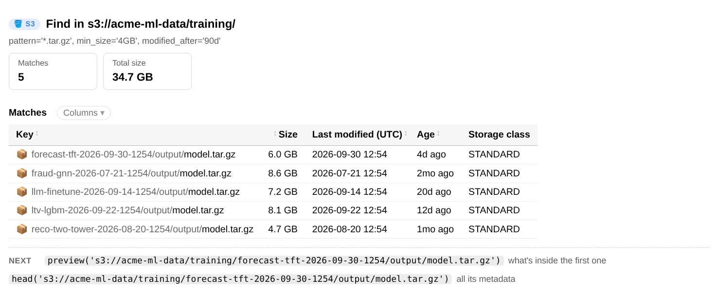
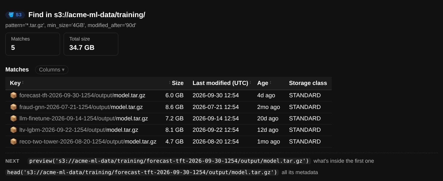
Model artifacts over 4 GB from the last 90 days.
| Filter | Matches | Example |
|---|---|---|
pattern |
Glob on the file name, or on the whole key if the pattern contains / |
"*.csv", "raw/*/2025-*" |
regex |
Regular expression searched in the whole key | r"/dt=2025-09-\d\d/" |
extensions |
File types; "csv" also matches .csv.gz |
["parquet", "csv"] |
min_size, max_size |
Size limits | "100MB", 5 * 1024**3 |
modified_after, modified_before |
Last-modified time | "7d", "2025-01-01" |
storage_classes |
Storage class | "GLACIER", ["STANDARD_IA", "ONEZONE_IA"] |
limit |
Stop after this many matches (default 1000; None for all) |
50 |
Biggest, newest, oldest, and one object's details
ui.largest("s3://acme-ml-data/", 10)
ui.newest("s3://acme-ml-data/raw/", 5)
ui.oldest("s3://acme-ml-data/")
ui.head("s3://acme-ml-data/curated/features/churn/train.parquet")   # every metadata field and tag
ui.link("s3://acme-ml-data/curated/features/churn/train.parquet", expires=900)   # download link, valid 15 min
Download a file or a folder
download() copies a file, or a whole folder with its sub-folders, to the notebook's disk with a progress bar, and says where it went. For a table file it also shows the pandas call that opens it. A file already downloaded (same size and time) is skipped, so if a big download stops, run it again to pick up where it left off. Files in GLACIER or DEEP_ARCHIVE are listed as needing a restore, and nothing starts if the disk doesn't have room.
Downloads go into the downloads folder, s3-downloads next to the notebook, unless you give a path:
ui.download("s3://acme-ml-data/curated/features/churn/train.parquet")        # s3-downloads/train.parquet
ui.download("s3://acme-ml-data/curated/features/churn/")                    # s3-downloads/churn/, sub-folders kept
ui.download("s3://acme-ml-data/curated/features/churn/", "/tmp/churn")     # somewhere else
To get a folder onto your own computer, download_zip() packs it into one .zip. It first checks that this notebook can make it, and downloads nothing if a check fails:
- Size and file count: at most
max_sizeof files (100 MB by default) andmax_filesfiles (10,000). It stops counting atmax_files, so the answer comes quickly even on a huge folder. - Disk space: the zip has to fit where it's written.
- Memory: files stream into the zip, so only a few MB are held at a time; it shows what's free.
- Read access: it reads one byte of one file, which fails if the role lacks
s3:GetObject(orkms:Decryptfor SSE-KMS files).
When a check fails, the report says what to change, such as the max_size= that would fit. Files in GLACIER or DEEP_ARCHIVE are left out and listed. Parquet, gzip and image files go in as they are, since compressing them again gains nothing; the rest are compressed. Once it's written, right-click the zip in JupyterLab's file browser (in s3-downloads) and choose Download.
ui.download_zip("s3://acme-ml-data/curated/features/churn/", dry_run=True)   # only the checks
ui.download_zip("s3://acme-ml-data/curated/features/churn/")                 # s3-downloads/churn.zip, if under 100 MB
ui.download_zip("s3://acme-ml-data/reports/", "/tmp/reports.zip", max_size="1GB")
To zip some files and not the whole folder, pass a list of files and folders from one bucket. They go in laid out as they are under the folder they share, and the zip is named after that folder and how many there are:
ui.download_zip([
    "s3://acme-ml-data/curated/features/churn/train.parquet",
    "s3://acme-ml-data/curated/features/fraud/train.parquet",
])   # features-2-files.zip, holding churn/train.parquet and fraud/train.parquet
In the S3 explorer, tick the files and click ⬇ Download selected instead.
The downloads folder, and cleaning it up
Everything download() and download_zip() save without a path goes in one folder, s3-downloads next to the notebook, so downloads don't mix with your notebooks and code. It's made with the first download, with a .gitignore that keeps it out of git and marks it as a folder clean_downloads() may empty (JupyterLab's file browser hides it).
downloads() shows what's there: each file, folder and zip with its size and when it was downloaded, how much of the disk they take, and what's free. Findings point out zips a stopped download_zip() left unfinished (churn.zip.part, after a kernel restart), a disk running out of room, and downloads over a month old, each with the clean_downloads() call that deletes them.
clean_downloads() deletes them to free the disk: everything, the ones you name, or what was downloaded before a date. The files are still in S3, so download() gets them again.
ui.downloads()                                # what's downloaded, and how much disk it takes
ui.clean_downloads(dry_run=True)              # what would go, deleting nothing
ui.clean_downloads("churn.zip")               # one download, by the name downloads() shows ("churn" for a folder)
ui.clean_downloads(older_than="7d")           # what was downloaded before this week
ui.clean_downloads()                          # all of them
To use another folder, pass downloads= (a path from the notebook's folder, or ~/... or an absolute path). The explorer's ⚙ changes the same setting.
ui = S3View(downloads="~/scratch/s3") # or ui.core.downloads = "~/scratch/s3"
clean_downloads() only empties a folder made for downloads: one that didn't exist (or was empty) when the first download went in. If you point downloads= at a folder that already held your own files, or at the notebook's own folder ("."), downloads still go there, but clean_downloads() refuses and downloads() says why, so it never deletes files it didn't download.
What's in a folder
summary() reads the listing once and gives you a dashboard: totals, estimated monthly cost, a breakdown by folder, file type and storage class, how old and how big the files are, and the largest files. At the top are plain-language findings, such as too many small files, data waiting to be restored from Glacier, cold data you could store more cheaply, and tiny files billed at a minimum size.
ui.summary("s3://acme-ml-data/")
ui.summary("s3://acme-ml-data/raw/", folder_depth=2, top_n=20)   # break down two folder levels, top 20 largest
ui.summary("s3://acme-ml-data/", limit=100_000)                  # stop after 100,000 keys (a quick sample)
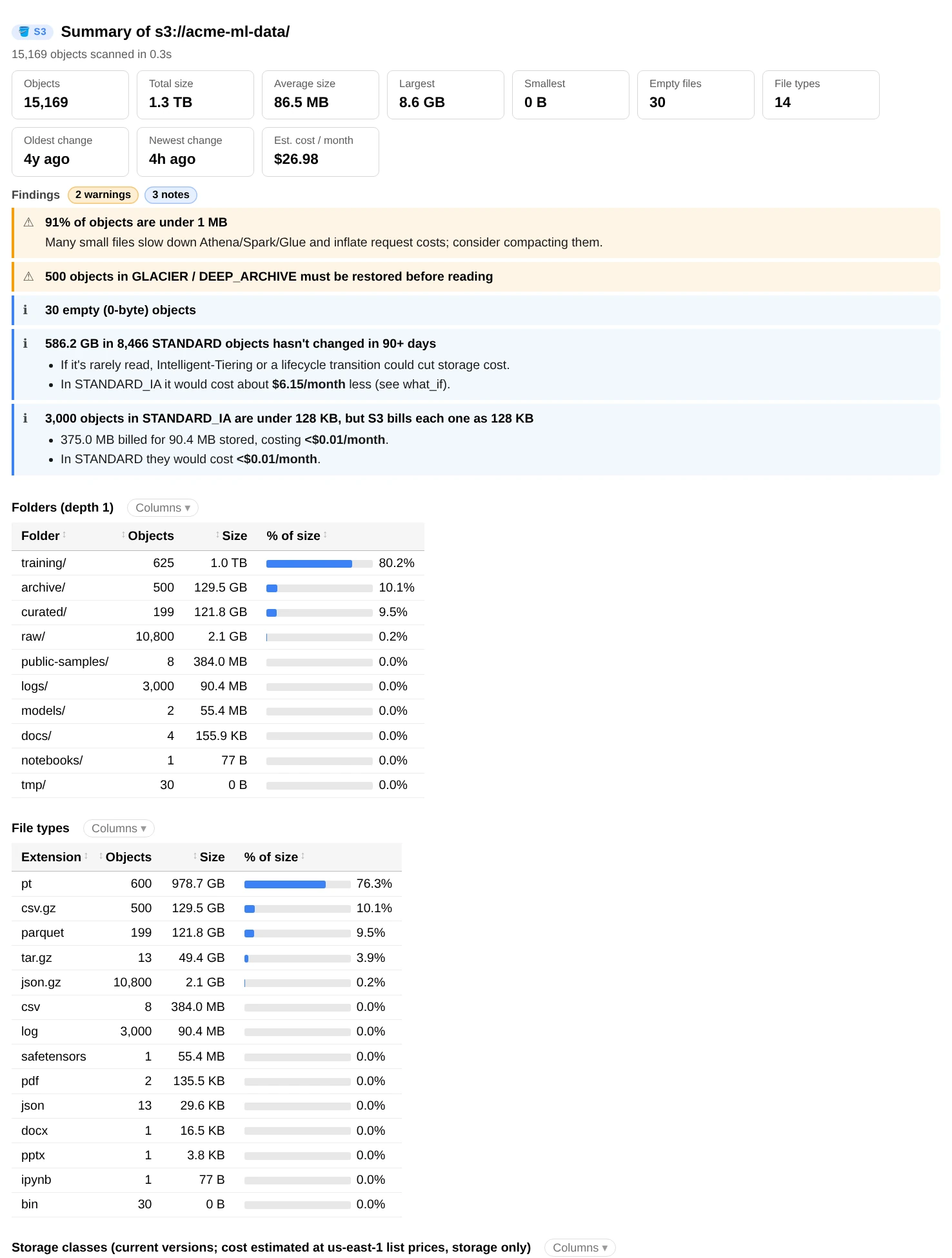
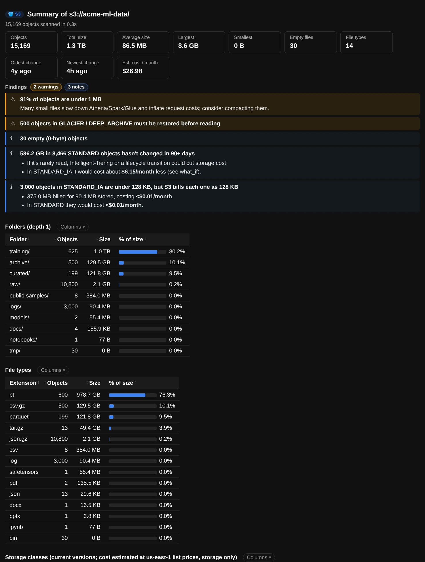
The top of ui.summary("s3://acme-ml-data/"). Further down: size and age histograms and the largest objects.
Look inside files
preview() shows what's in a file without downloading all of it: the first rows of a table and its schema, the files inside an archive, a model's tensors, a notebook's cells, and more. It picks the reader from the file name, or from the file's first bytes when there's no extension (Spark's part-00000, Firehose output) or the wrong one.
ui.preview("s3://acme-ml-data/curated/features/churn/train.parquet", n=8)   # first 8 rows
ui.preview("s3://acme-ml-data/training/churn-xgb-2025-09-01-1030/output/model.tar.gz")
ui.preview("s3://acme-ml-data/models/tiny-llm/model.safetensors")
ui.preview("s3://acme-ml-data/models/tiny-llm/config.json")
ui.preview("s3://acme-ml-data/notebooks/churn-data-checks.ipynb")
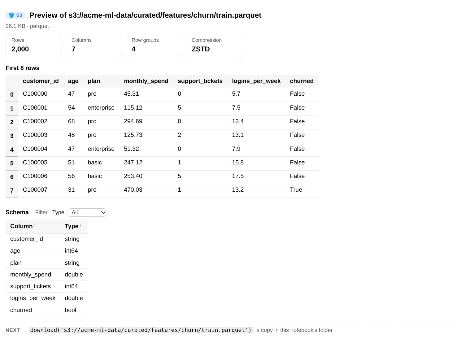
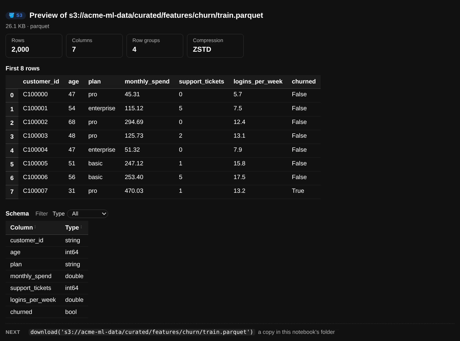
A Parquet file: only the footer and the first row group are downloaded.
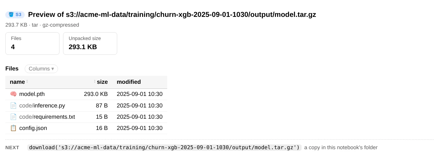
A SageMaker model.tar.gz, listed without extracting it.
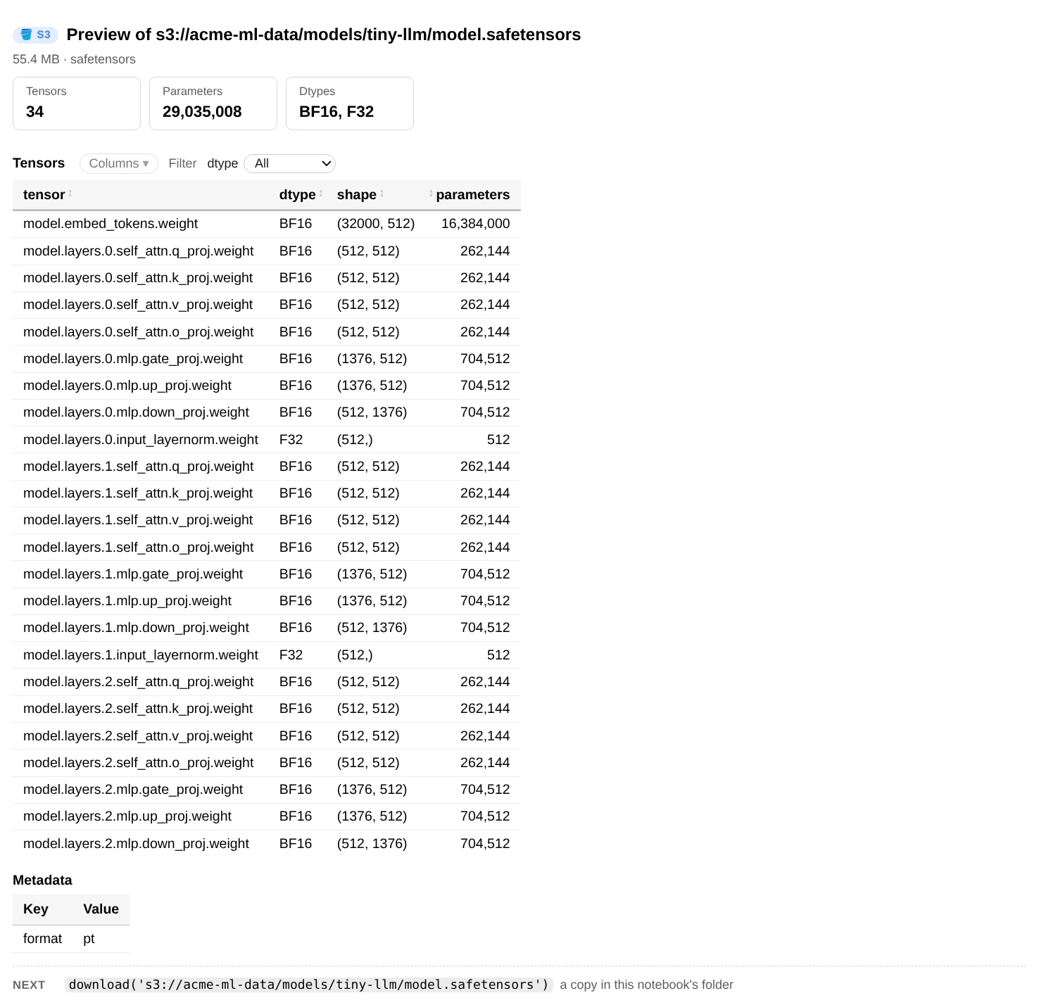
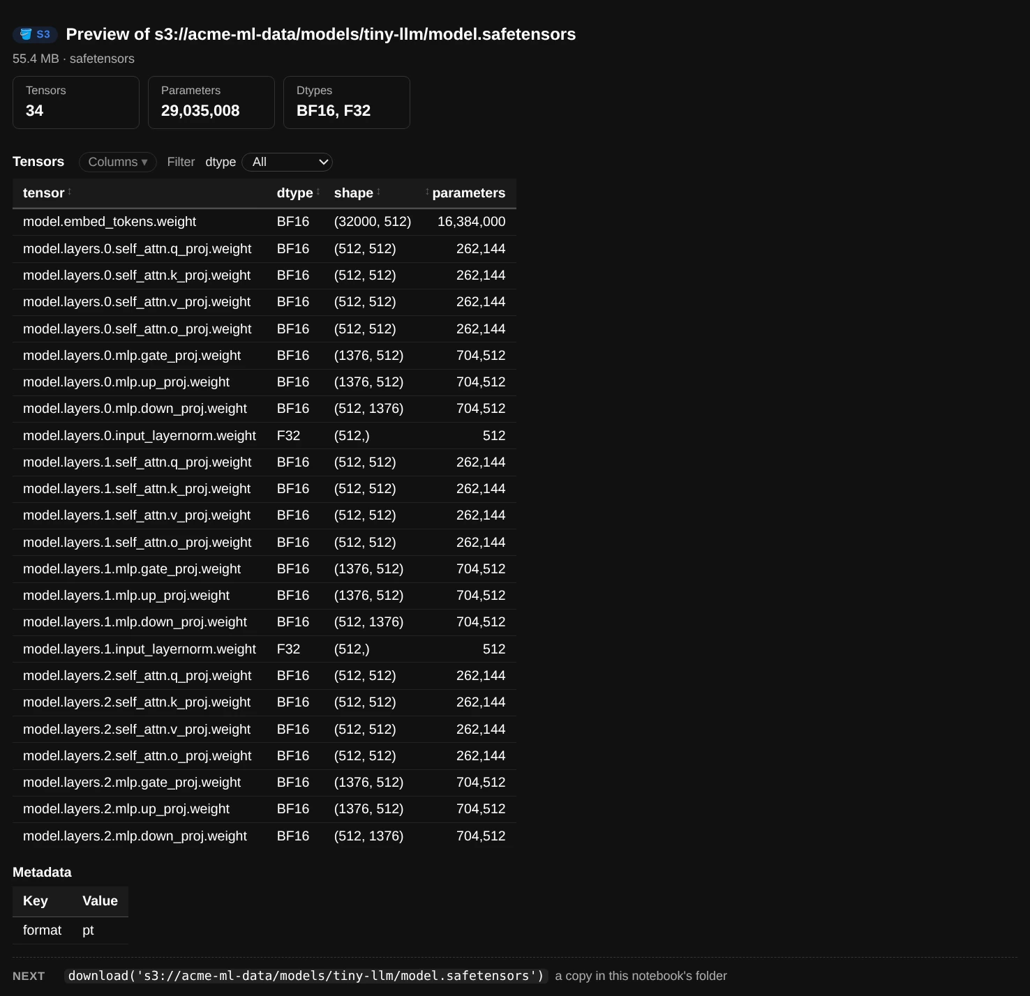
A .safetensors model: only its header is read, so this is instant even for a multi-GB file.
A JSON file that isn't a list of records shows as a tree, coloured like code. Click a line to fold or unfold it. Hover over a line to see the Python that reaches it (data['sagemaker']['hyperparameters']), where data = ui.core.read_json(...) loads the file. The tree starts with as much open as fits on a screen. In a long list of records only the first is open, and the rest show one line each. A string that holds JSON (SageMaker hyperparameters, an SNS message, an SQS body) shows as the JSON inside it. A long string folds to its start, and a click shows the whole text with its line breaks. Arrays show their first n items. A file bigger than the 512 KB preview window shows its start, marked as such, instead of a page of raw text.
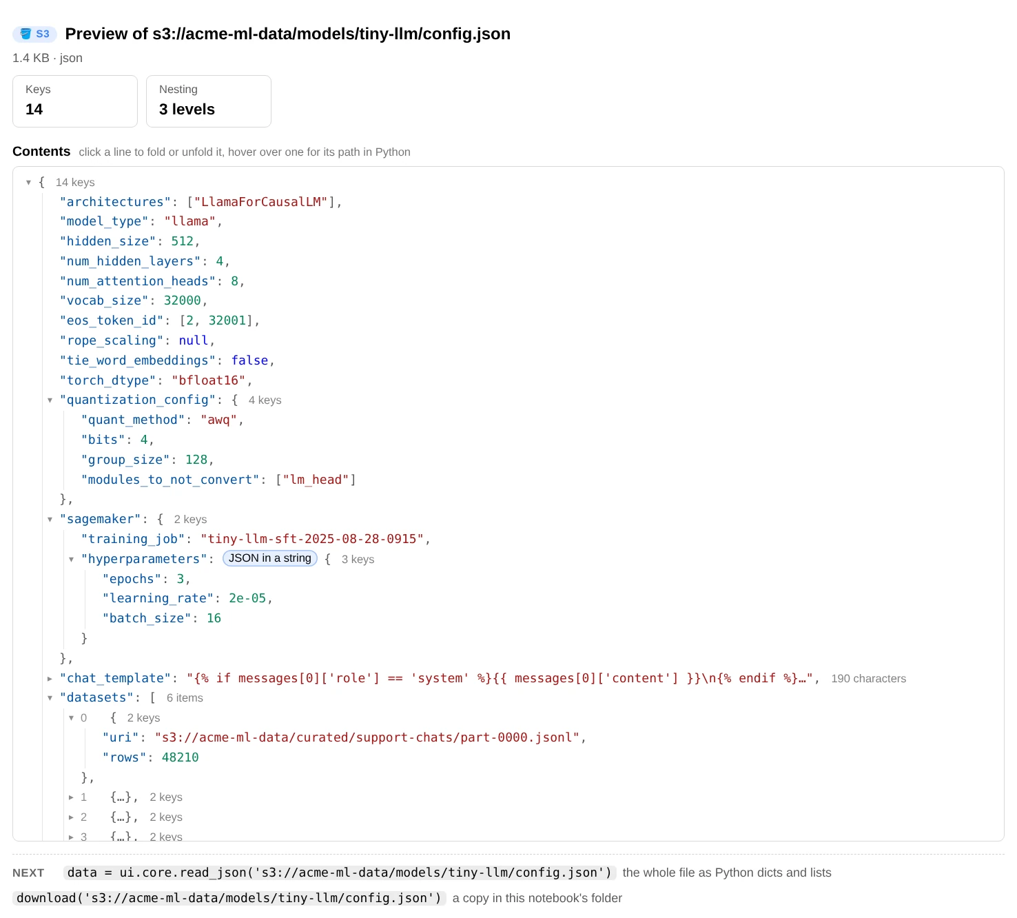
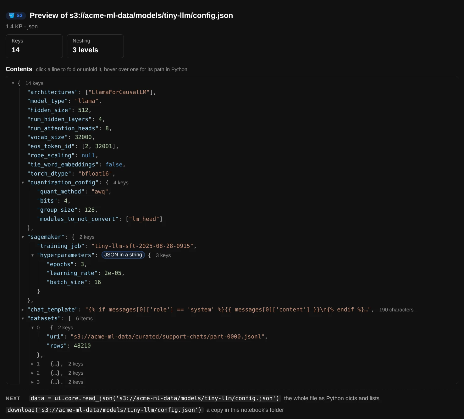
A model's config.json as a tree: each object and array folds under a click, and each line's tooltip is its path in Python.
Supported file types
| Kind | Extensions | preview() shows |
read_df() |
|---|---|---|---|
| Delimited text | .csv .tsv .psv |
First rows | ✓ |
| JSON | .json .jsonl .ndjson |
A table of records, or a tree you fold with a click, coloured like code. A string holding JSON is shown unpacked, and a file too big to read whole shows its start | ✓ |
| Columnar | .parquet .orc .feather .arrow |
First rows, schema and row count; reads only what it needs | ✓ |
| Avro | .avro |
First rows, schema and codec (built-in reader; snappy needs python-snappy) |
✓ |
| Excel | .xlsx .xlsm .xls |
Sheet names and first rows (needs openpyxl; .xls needs xlrd) |
✓ sheet_name= |
| NumPy | .npy .npz |
Shape, dtype and first rows, or the arrays inside | ✓ .npy, up to 2-D |
| Archives | .zip .tar .tar.gz .tgz |
The files inside | |
| Models | .safetensors .pt .pth .ckpt .pkl .joblib |
Tensors and parameter count, or the files in a checkpoint. Pickles are never loaded, because unpickling can run code | |
| Notebooks | .ipynb |
Kernel and a list of cells | |
| Images, audio, video | .png .jpg .gif .webp, .wav .mp3 .flac, .mp4 .webm .mov |
The image, or a player | |
.pdf |
The first three pages as they look, scanned pages too (needs pypdfium2 and pillow), with the page count, title and first page's text (needs pypdf); without either, a link. Every page with ui.document() |
||
| Word | .docx .docm .dotx |
The first paragraphs laid out as in the document: headings, lists, tables and pictures in place; word count (no package needed) | |
| PowerPoint | .pptx .pptm .ppsx |
Every slide's title and text, and which have speaker notes (no package needed) | |
| Old Office | .doc .ppt .msg |
Recognised, with how to convert them to .docx / .pptx (their binary format can't be read here) |
|
| Text | .txt .log .md .yaml .xml .sql .py and more |
First lines |
Any of them can also be compressed: .gz, .bz2, .xz, or .zst (Python 3.14+, or pip install zstandard). Anything else is shown as text or a hex dump.
What's inside many files at once
preview() opens one file. file_details() looks inside every file under a prefix and puts each kind in its own table: a PDF's pages, title and author and whether it has text, a Word file's words and headings, a deck's slides, each Excel sheet's size, a table's rows and column names, a picture's width and height, a video's length, the files in an archive. It reads only the parts each format needs, in 256 KB ranged requests: a PDF's page tree and first three pages, a parquet footer, a picture's first bytes, the first 256 KB of a CSV. It stops at max_read (1 GB by default) and says how much it read.
ui.file_details("s3://acme-ml-data/docs/")                       # every file, up to limit=200 in key order
ui.file_details("s3://acme-ml-data/docs/", extensions="pdf")     # only the PDFs: pages, text, title, author
ui.file_details("s3://acme-ml-data/curated/", pattern="*.parquet", limit=None, max_read="5GB")
ui.file_details("s3://acme-ml-data/docs/model-card-churn-xgb.docx")   # one file
ui.ls("s3://acme-ml-data/docs/", details=True)                   # one level, with a "What's inside" column

report = ui.core.file_details("s3://acme-ml-data/docs/", extensions="pdf")
df = report.to_df()                                # one row per file: format, size, summary, pages, title, ...
df[df.text == False]                               # the scanned PDFs
The findings point out what to act on: scanned PDFs with no text, which need OCR before their words can be searched or sent to a model; PDFs that need a password; files whose content isn't what their name says (an HTML error page saved as report.pdf, parquet saved as .csv); parquet or CSV files in one folder whose columns differ, which breaks Athena, Glue and Spark tables; pictures in mixed sizes; and files it couldn't read, with why. Counts that come from the start of a file are marked: ≈ for an estimate (a CSV's rows from its first 256 KB) and + for a lower bound (a compressed CSV).
| Kind | What file_details() reports |
What it reads |
|---|---|---|
| Pages, whether the first 3 pages have text (none = probably scanned), page size (A4, Letter, …), title, author, the app that made it, creation date, PDF version, whether it needs a password | The page tree and the first 3 pages (needs pypdf) |
|
| Word | Words, pages (as Word last saved them), headings, tables, pictures, title, author, when it was last saved | The document's text (no package needed) |
| PowerPoint | Slides, words, slides with speaker notes, tables, pictures, title, author | The slides' text |
| Excel | Each sheet's name and rows × columns (header row included), title, author | The size Excel saves at the top of each sheet |
| Parquet | Rows, column names, row groups, compression, the program that wrote it | The footer (needs pyarrow) |
| ORC, Feather | Rows, column names, compression, stripes or record batches | The metadata (needs pyarrow) |
| Avro | Rows, column names, codec | Block headers, in files up to 64 MB |
| CSV, TSV, PSV, JSON lines | Column names (the header, or the first record's keys), rows: exact up to 256 KB, then estimated (≈), or a lower bound when compressed (+) |
The first 256 KB |
| JSON | Records and their keys, or an object's keys; JSON lines saved as .json are recognised |
The whole file, up to 16 MB |
| Pictures | Format (PNG, JPEG, GIF, BMP, WebP, TIFF) and width × height | The first 64 KB |
| Audio, video | Length; sample rate and mono / stereo (WAV, FLAC); width × height (MP4, MOV). An MP4 with no index is flagged as cut off | The header, or the MP4 moov box |
| Archives | Files inside and their unpacked size | A zip's index, or a tar's headers |
| Models, arrays | Tensors, parameters and dtypes (.safetensors); shape and dtype (.npy); arrays (.npz); files inside a PyTorch checkpoint. Pickles are never loaded |
Headers only |
| Notebooks | Cells, code cells, outputs, kernel | The whole file, up to 50 MB |
| Text | Lines, exact or estimated | The first 256 KB |
| Old Office | Recognised, with how to convert it | Nothing |
Every file's format is checked against its first bytes, so a file with no extension (Spark's part-00000) is still described, and a wrong one is flagged. A file is read for at most 128 MB, and files in GLACIER or DEEP_ARCHIVE are skipped with the restore command to run. Without pypdf or pyarrow, those files are listed with what to install.
Load files into Python
ui.core is the analyzer behind the view. Its readers return data instead of printing it.
s3 = ui.core

df = s3.read_df("s3://acme-ml-data/curated/features/churn/train.parquet")
df = s3.read_df("s3://acme-ml-data/curated/features/churn/train.parquet", nrows=1000, columns=["age", "plan"])
df = s3.read_df("s3://acme-ml-data/raw/events/dt=2025-09-01/part-00000.json.gz", fmt="jsonl", nrows=500)   # one record per line
df = s3.read_df("s3://acme-ml-data/reports/q3.xlsx", sheet_name="Summary")       # Excel: needs openpyxl
df = s3.read_df("s3://acme-ml-data/spark-output/part-00000", fmt="parquet")     # no extension: say what it is
df = s3.read_df("s3://acme-ml-data/exports/data.txt", fmt="csv", sep=";")        # extra options go to pandas
s3.read_lines("s3://acme-ml-data/logs/app/2025/09/01/app-00001.log", 50)   # first 50 lines
s3.read_json("s3://acme-ml-data/config/settings.json")
s3.read_jsonl("s3://acme-ml-data/raw/events/dt=2025-09-01/part-00000.json.gz", n=100)
s3.read_avro("s3://acme-ml-data/kafka/events.avro", n=100)          # a list of dicts
s3.read_npy("s3://acme-ml-data/embeddings/vectors.npy", nrows=10)    # a NumPy array
s3.parquet_info("s3://acme-ml-data/curated/features/churn/train.parquet")   # rows, row groups, schema
s3.list_archive("s3://acme-ml-data/training/churn-xgb-2025-09-01-1030/output/model.tar.gz").entries
s3.safetensors_info("s3://acme-ml-data/models/tiny-llm/model.safetensors")["tensors"]

with s3.open("s3://acme-ml-data/raw/events/dt=2025-09-01/part-00000.json.gz") as f:   # a stream, decompressed
    first_line = f.readline()

s3.download("s3://acme-ml-data/training/churn-xgb-2025-09-01-1030/output/model.tar.gz", "/tmp/")
s3.download_folder("s3://acme-ml-data/curated/features/churn/", "/tmp/churn")   # every file, sub-folders kept
s3.plan_zip("s3://acme-ml-data/curated/").can_download   # would download_zip() work here? (downloads nothing)
s3.list_downloads().to_df()                               # what's in the downloads folder (s3.downloads_folder())
s3.clean_downloads(older_than="30d", dry_run=True).freed  # bytes it would free
For worked examples that load a JSON export, a CSV, an Excel workbook or a whole folder and build on it, see Build your own analysis.
Read PDFs, Word and PowerPoint files
preview() gives a quick look: a Word file laid out with its headings, lists, tables and pictures in place, and a PDF's first three pages as they look (click a page to see it as big as the notebook, with ‹ › to step through the pages). ui.document() shows the whole thing: a Word file the same way, a deck slide by slide, and a PDF's text laid out to read, like a web page. Its headings come from the font sizes, its paragraphs are joined back up from the PDF's lines (with words split at the end of a line made whole), its bullet and numbered lists are lists, and a thin line marks where each page starts. The running headers, footers and page numbers are left out, and a note says which. Word and PowerPoint files are read with Python's standard library. A PDF's text needs pypdf, and drawing its pages needs pypdfium2 and pillow (%pip install pypdf pypdfium2 pillow).
ui.preview("s3://acme-ml-data/docs/model-card-churn-xgb.docx")        # the first paragraphs, pictures in place
ui.preview("s3://acme-ml-data/docs/q3-ml-platform-review.pptx")       # every slide's title and text
ui.preview("s3://acme-ml-data/docs/invoices/vendor-invoice-0471.pdf") # the first pages as they look
ui.document("s3://acme-ml-data/docs/data-retention-policy.pdf")       # its text, laid out to read
ui.document("s3://acme-ml-data/docs/data-retention-policy.pdf", pages=[2])       # just page 2
ui.document("s3://acme-ml-data/docs/data-retention-policy.pdf", pictures=True)   # every page drawn, text underneath
ui.document("s3://acme-ml-data/docs/data-retention-policy.pdf", pictures=False)  # text only, scanned pages too
ui.document("s3://acme-ml-data/docs/q3-ml-platform-review.pptx", pages=[2, 3])   # slides 2-3, with speaker notes
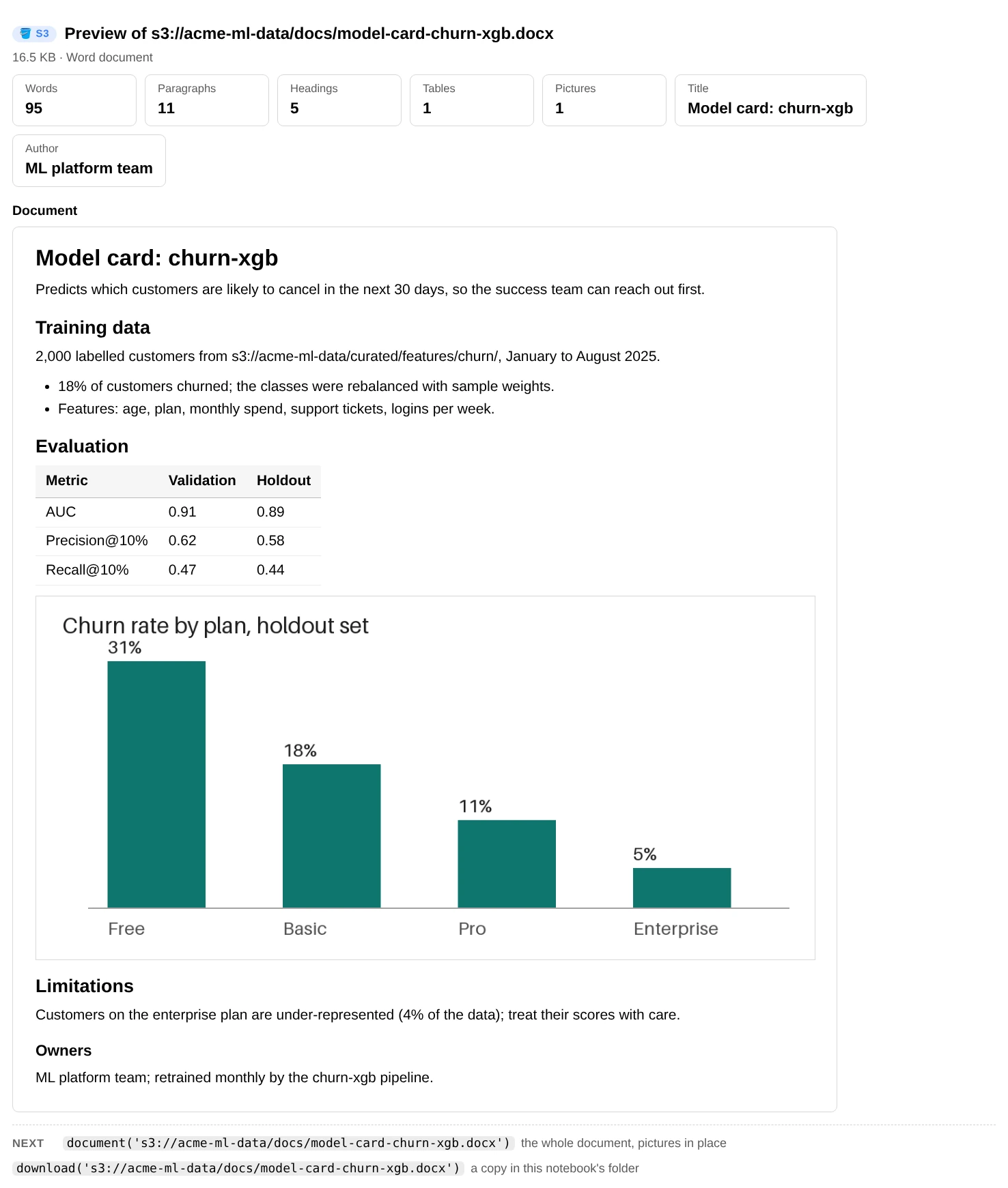
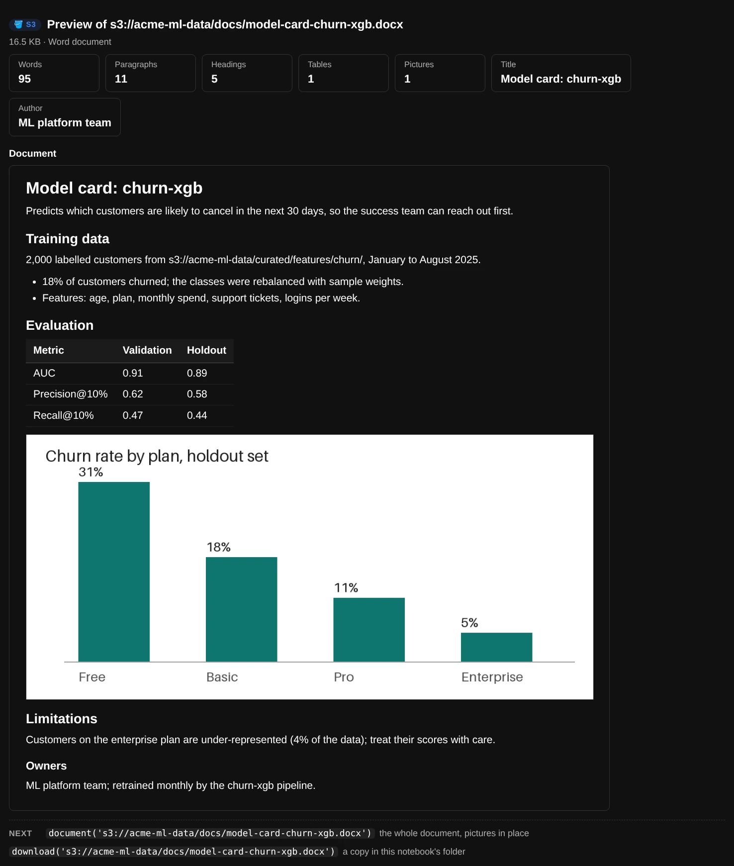
A Word model card, laid out as it reads: headings, bullets, the table and the chart where the author put them.
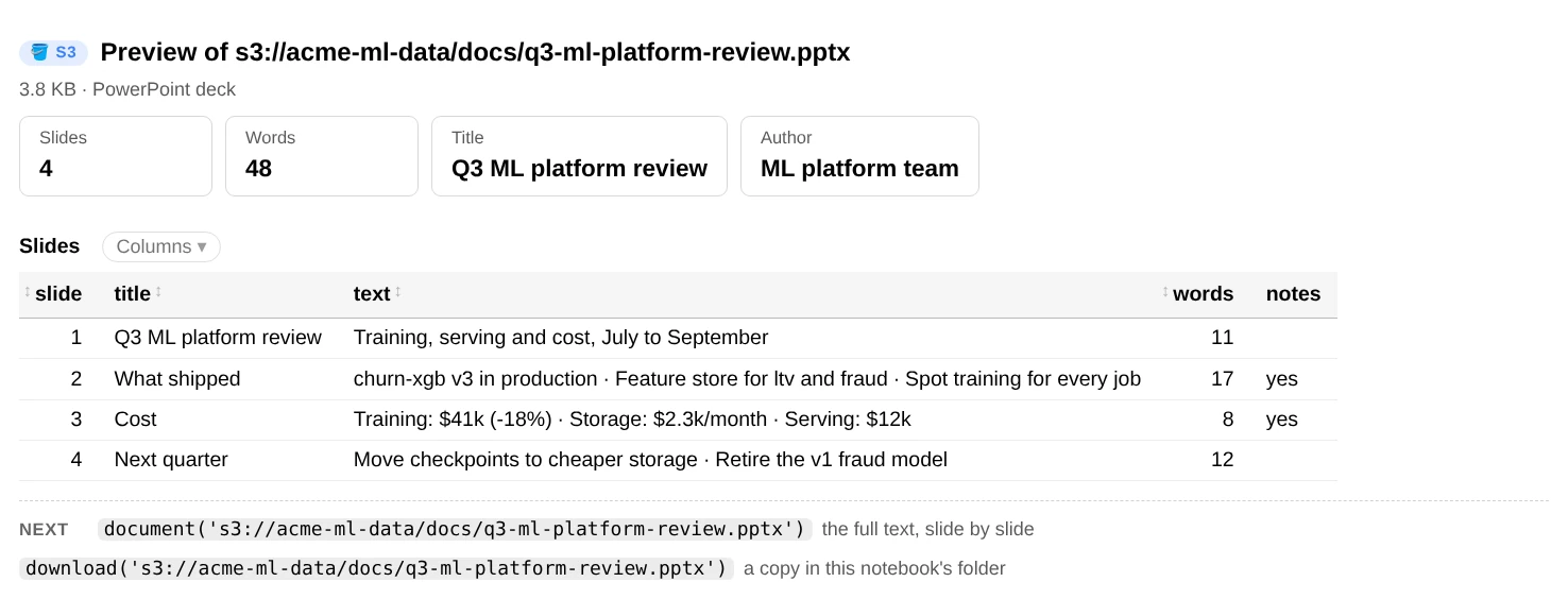
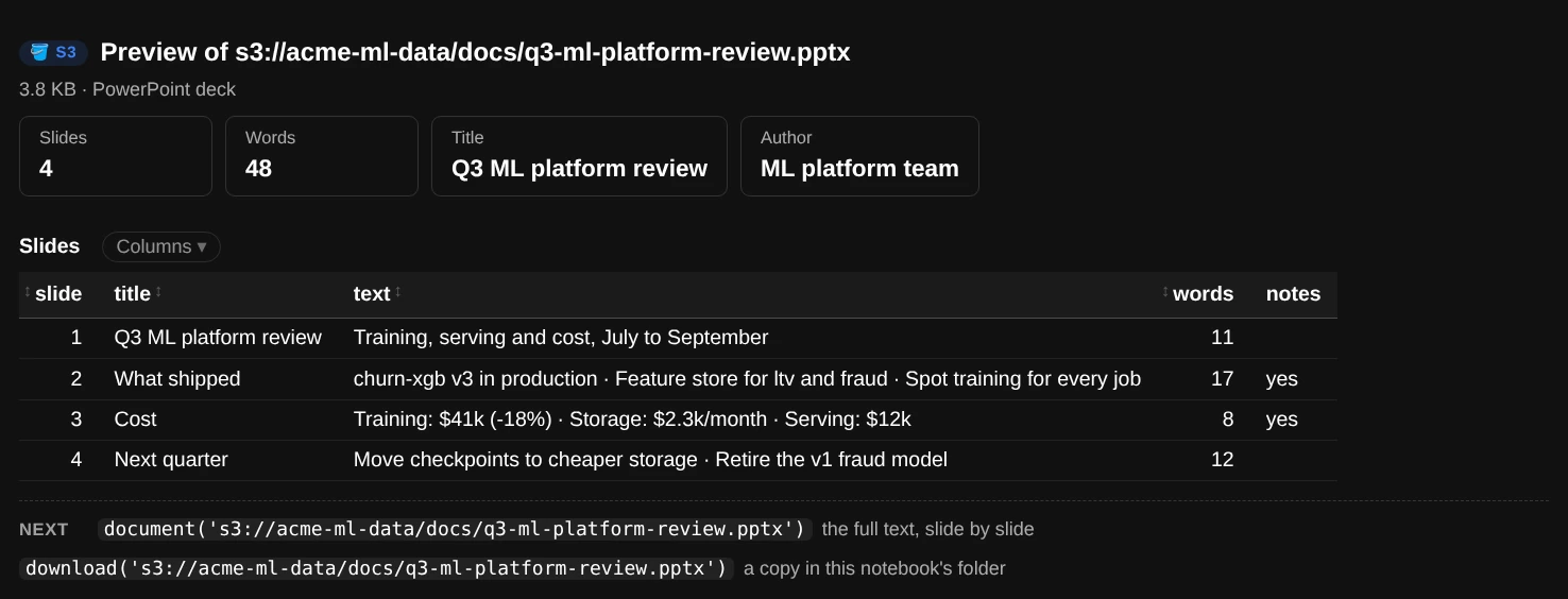
A PowerPoint deck, in the order it's presented.
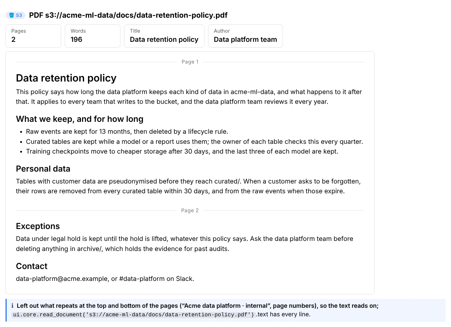
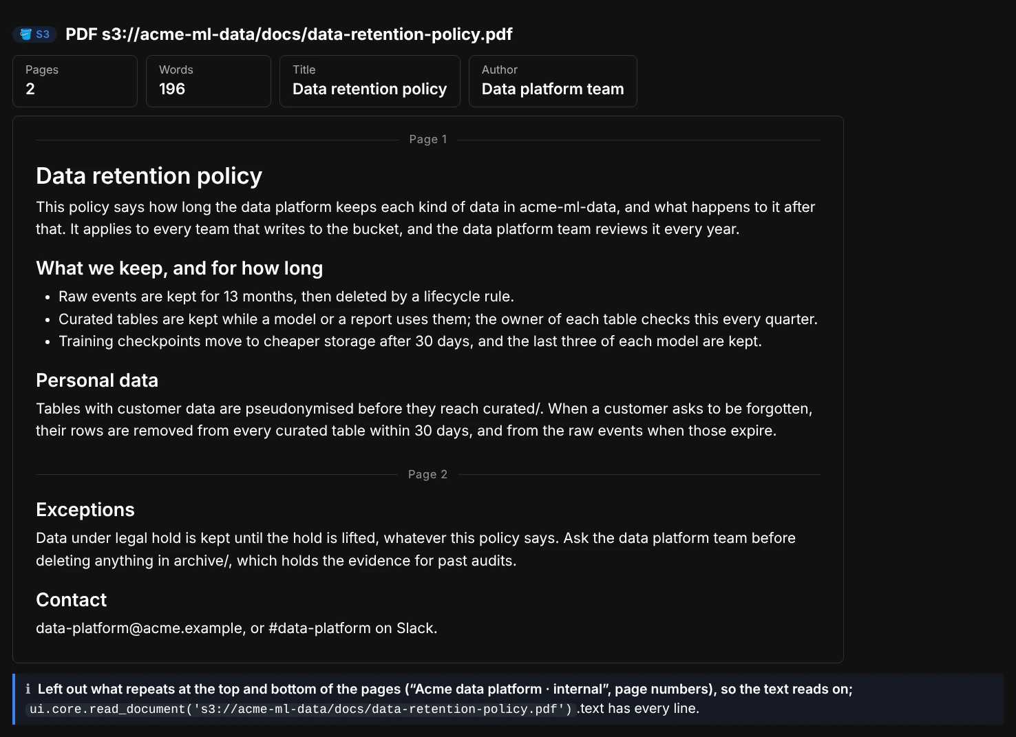
ui.document(...) on a two-page PDF: its text laid out to read, the lines of each paragraph joined back up, without the header and page numbers on every page.
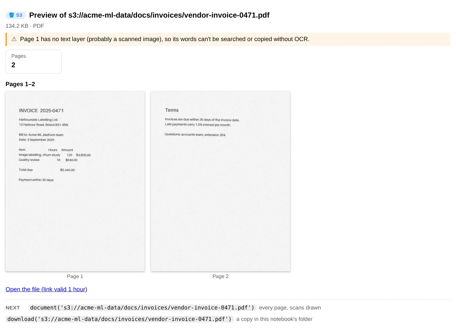
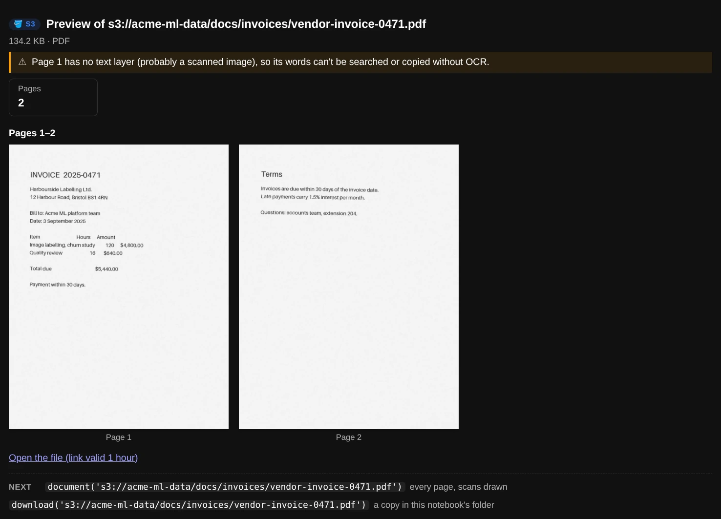
A scanned invoice has no text to show, so the preview draws its pages. ui.document(...) shows them full width.
To use the text in Python (for search, summaries, or checking what a knowledge base will ingest), read_document() returns a Document:
doc = ui.core.read_document("s3://acme-ml-data/docs/data-retention-policy.pdf")
doc.text                  # everything, pages separated by blank lines
doc.parts                 # one string per page (PDF) or slide (PowerPoint); paragraphs and tables for Word
doc.numbers               # the page / slide number of each part
doc.page_count, doc.word_count, doc.title, doc.author

deck = ui.core.read_pptx("s3://acme-ml-data/docs/q3-ml-platform-review.pptx")
deck.slide_titles, deck.notes                     # per slide
card = ui.core.read_docx("s3://acme-ml-data/docs/model-card-churn-xgb.docx")
card.headings, card.tables                        # [(level, text)], tables as rows of cells
ui.core.read_pdf("s3://acme-ml-data/docs/data-retention-policy.pdf", pages=range(1, 3))

from aws_analyzer.s3 import pdf_flow, pdf_furniture
doc = ui.core.read_pdf("s3://acme-ml-data/docs/data-retention-policy.pdf", layout=True)
doc.layout[0].lines[0]    # PdfLine(text='Data retention policy', x=72.0, y=92.0, size=20.0, bold=True)
pdf_flow(doc)             # [('page', 1), ('title', 'Data retention policy'), ('p', 'This policy says ...'), ...]
pdf_furniture(doc)        # ['Acme data platform · internal', 'page numbers']: what pdf_flow leaves out
pages = ui.core.render_pdf("s3://acme-ml-data/docs/invoices/vendor-invoice-0471.pdf")   # [Picture], one per page
pages[0]                                          # shows the page in the notebook; pages[0].data is the PNG / JPEG
card = ui.core.read_docx("s3://acme-ml-data/docs/model-card-churn-xgb.docx", pictures=True)
card.pictures                                     # the pictures, in reading order, each with its alt text

texts = {obj.key: ui.core.read_document(obj.uri).text                  # every PDF under a folder
         for obj in ui.core.find("s3://acme-ml-data/docs/", extensions="pdf")}
A PDF has no paragraphs or headings of its own, only lines of text placed on a page, so ui.document() and pdf_flow work them out from where each line sits, how big it is and whether it's bold. That reads well for most documents, but lists drawn as shapes (as browsers print web pages) read as one paragraph, and a table reads as one line per row. ui.core.read_document(uri).text has every line as pypdf reads it, and pictures=True shows the pages as they look. Scanned PDFs are images with no text layer: their text comes back empty and the preview says so, but preview() and ui.document() draw those pages, so you can still read them. Searching or copying their words needs OCR (for example Amazon Textract). Pictures in Word files show where they are in the text; formats browsers can't show (EMF and WMF, which Word uses for some charts) are named instead. One report shows at most 20 pages or pictures, so the notebook stays small. Password-protected PDFs: pass password="...". Old .doc / .ppt files use a binary format this tool can't read; save them as .docx / .pptx, or convert them with LibreOffice: soffice --headless --convert-to docx FILE.doc.
Cut storage costs
Costs appear throughout: summary() prices the files in a folder, bucket_info() and overview() price whole buckets (old versions included), and versions() and uploads() price the storage you can't see in a normal listing. They're estimates of storage only, at us-east-1 list prices, and follow S3's billing rules: STANDARD_IA, ONEZONE_IA and GLACIER_IR bill at least 128 KB per file, and GLACIER and DEEP_ARCHIVE add 40 KB of index data per file.
Preview a lifecycle rule before you add it
what_if() shows what a lifecycle rule would do if it ran today: how many files it would move or delete, the monthly cost before and after, the one-time cost (transition requests, and early-deletion charges for files that haven't reached their storage class's minimum duration), and how soon it pays for itself. It follows S3's own rules, for example that files under 128 KB aren't moved. It also prints the rule, ready to add.
ui.what_if("s3://acme-ml-data/training/", move_after={30: "STANDARD_IA", 180: "GLACIER"})
ui.what_if("s3://acme-ml-data/logs/", move_after=30, to="STANDARD_IA")
ui.what_if("s3://acme-ml-data/tmp/", delete_after=7)
ui.what_if("s3://acme-ml-data/raw/", move_after=0, to="INTELLIGENT_TIERING")
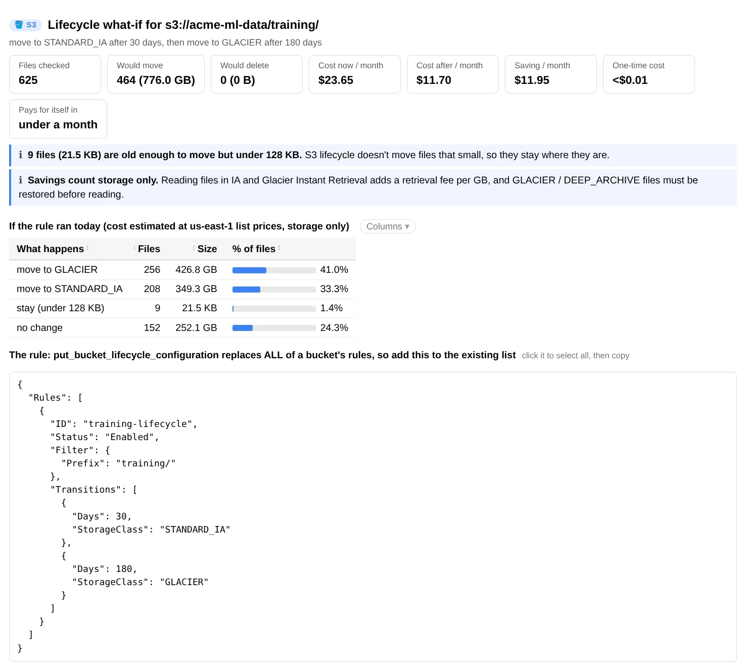
Moving training outputs to STANDARD_IA after 30 days and to GLACIER after 180.
To add the rule yourself (the tool never changes your buckets):
import boto3

impact = ui.core.simulate_lifecycle("s3://acme-ml-data/training/", move_after={30: "STANDARD_IA", 180: "GLACIER"})
print(f"saves ${impact.monthly_savings:,.2f} a month")
client = boto3.client("s3")
current = client.get_bucket_lifecycle_configuration(Bucket="acme-ml-data")["Rules"]
# put_bucket_lifecycle_configuration replaces every rule, so send the existing ones too
client.put_bucket_lifecycle_configuration(Bucket="acme-ml-data",
                                          LifecycleConfiguration={"Rules": current + [impact.rule()]})
If the bucket has no lifecycle rules yet, get_bucket_lifecycle_configuration raises an error; use an empty list for current instead.
Hidden storage: old versions, unfinished uploads
ui.versions("s3://acme-ml-data/")                    # noncurrent versions and what they cost
ui.uploads("s3://acme-ml-data/")                     # unfinished multipart uploads: billed but invisible
Duplicate files
duplicates() finds files with identical content and tells you what their copies take and cost per month, which copy to keep, and which folders hold nothing but copies, such as a backfill of files that also exist elsewhere. It's read-only: it shows how to get the list, and deleting is up to you.
ui.duplicates("s3://acme-ml-data/public-samples/")                    # the usual call
ui.duplicates("s3://acme-ml-data/", min_size="1MB", max_read="50GB")  # skip small files, read more if needed
ui.duplicates("s3://acme-ml-data/", method="etag")                    # the listing only: reads no file
ui.duplicates("s3://acme-ml-data/models/", method="strict")           # hash every candidate with SHA-256
It does the cheap checks first and only reads what it has to:
- Size. A file no other file matches in size can't be a copy. This comes from the listing, so it's free.
- ETag. Files with the same size and ETag are copies: the ETag is S3's checksum of the content (the MD5, for a file uploaded in one part). Also free.
- SHA-256 of the content. A copy uploaded in parts of another size, or encrypted with SSE-KMS, gets a different ETag. So where files share a size but not an ETag, it reads one file per ETag: the first 64 KB, then the whole file only where those match. It reads at most
max_read(10 GB by default), starting where the saving could be biggest, and says how much it read and what it had to leave out.
For each group, Keep suggests a file you can read without a restore, in the folder with the fewest copies, then the oldest, so a folder of copies empties out. In a versioned bucket a deleted copy stays as a noncurrent version until a lifecycle rule removes it; the report says so. To act on the result in pandas:
report = ui.core.find_duplicates("s3://acme-ml-data/public-samples/")
df = report.to_df()              # one row per file: group, role ('keep' / 'copy'), key, size, sha256, ...
copies = df[df.role == "copy"]   # everything but the file to keep in each group
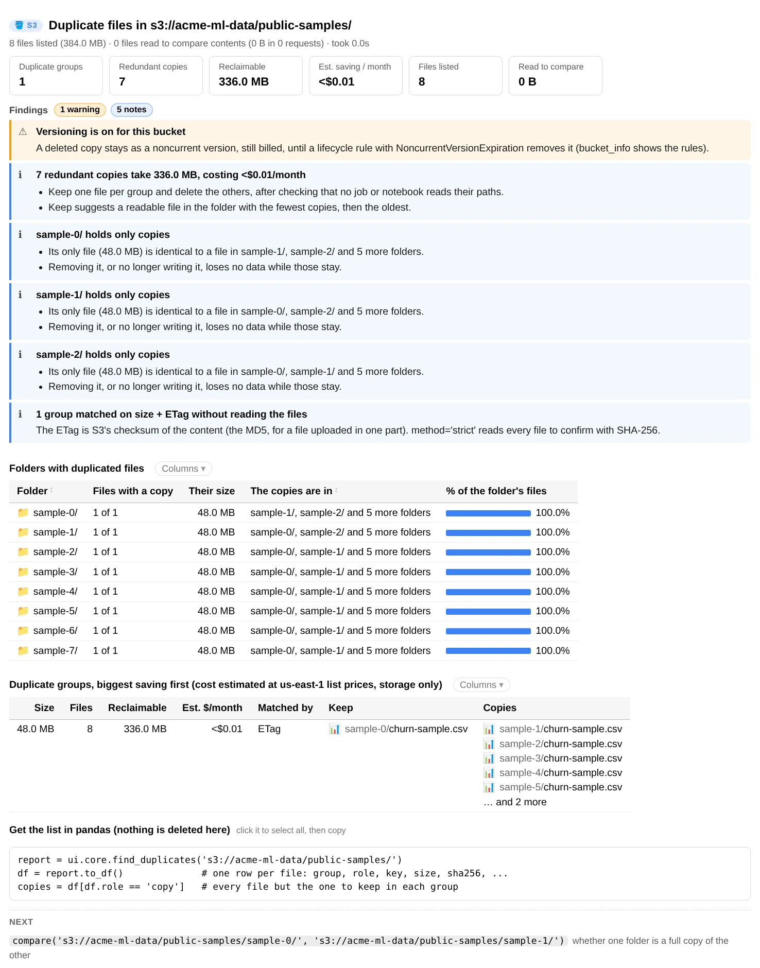
ui.duplicates(...): groups of identical files and the space their copies take.
Use your region's prices
The default prices are us-east-1 list prices for the first 50 TB, in USD per GB-month. Pass your own from the S3 pricing page; any class you leave out keeps its default.
from aws_analyzer import S3Analyzer, S3View

ui = S3View(S3Analyzer(prices={"STANDARD": 0.025, "STANDARD_IA": 0.0138}))
Recover deleted files
In a versioned bucket, deleting a file only adds a delete marker; the data is still there. deleted() lists those files, most recent first, with the size you'd get back and the code that restores one.
ui.deleted("s3://acme-ml-data/")
ui.deleted("s3://acme-ml-data/curated/", deleted_after="7d")    # only files deleted in the last week
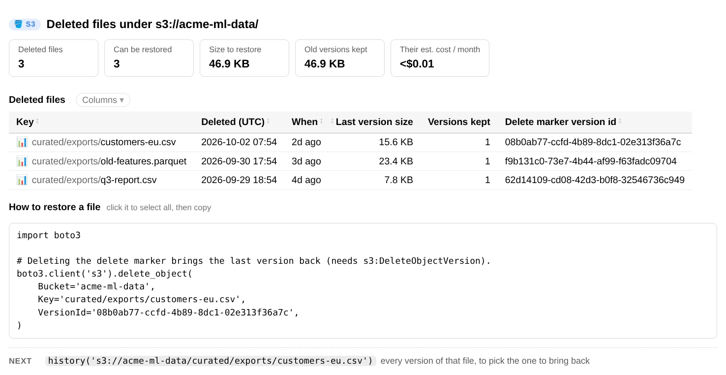
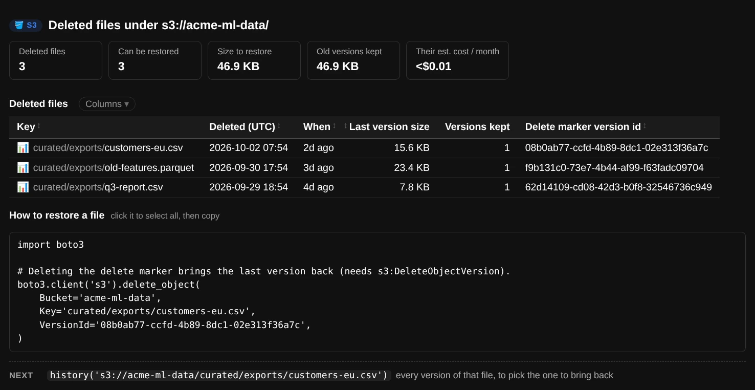
ui.deleted("s3://acme-ml-data/")
Restoring means deleting the delete marker, which needs s3:DeleteObjectVersion. To bring back everything deleted under a folder in the last day:
import boto3

client = boto3.client("s3")
for f in ui.core.deleted_files("s3://acme-ml-data/curated/exports/", deleted_after="1d").files:
    if f.restorable:
        client.delete_object(Bucket="acme-ml-data", Key=f.key, VersionId=f.marker_version_id)
For one file's full history, use ui.history("s3://acme-ml-data/curated/exports/q3-report.csv"). If versioning is off, deleted() says so: deleted files are gone for good in that case.
Check a copy or sync
compare() matches two prefixes by relative key, size and ETag, so you can check that a copy, sync or migration is complete.
ui.compare("s3://acme-ml-data/curated/", "s3://acme-eu-exports/curated/")

result = ui.core.compare("s3://acme-ml-data/curated/", "s3://acme-eu-exports/curated/")
result.in_sync, len(result.only_in_a), len(result.different)
Files encrypted with SSE-KMS, or uploaded with different multipart settings, have different ETags even when their content is identical. Pairs with the same size but multipart ETags are counted separately, as “ETag not comparable”.
Use the data in Python
Every report has a data version on ui.core (an S3Analyzer) that returns dataclasses, lists and DataFrames instead of printing. Use it to build your own checks, charts or scheduled jobs.
from aws_analyzer.s3 import explain_policy, objects_to_df

s3 = ui.core

summary = s3.summarize("s3://acme-ml-data/")          # PrefixSummary
summary.total_size, summary.monthly_cost               # bytes, USD per month
summary.by_extension["parquet"].size                   # bytes of parquet
{cls: stat.size for cls, stat in summary.by_storage_class.items()}

old_checkpoints = s3.find("s3://acme-ml-data/training/", extensions="pt", modified_before="180d")
df = objects_to_df(old_checkpoints)                    # key, size, last_modified, storage_class, extension, etag, uri
df.groupby("storage_class")["size"].sum()

for obj in s3.iter_objects("s3://acme-ml-data/raw/", limit=5000):   # stream a listing
    pass

cfg = s3.bucket_config("acme-ml-data")                 # BucketConfig
cfg.versioning, cfg.encryption, cfg.lifecycle_rules
reports = s3.bucket_reports(match="acme-*")            # config + CloudWatch size for many buckets
for st in explain_policy(s3.bucket_policy("acme-ml-data"), s3.account_id()):
    print(st.effect, st.who, st.actions, st.resources, st.conditions)
The analysis functions don't call AWS, so they also work on your own lists of files, for example rows from an S3 Inventory report:
from datetime import datetime, timezone
from aws_analyzer.s3 import ObjectInfo, simulate_lifecycle_objects, summarize_objects

rows = [ObjectInfo("acme-ml-data", "raw/a.json", 1_200_000, datetime(2025, 1, 5, tzinfo=timezone.utc)),
        ObjectInfo("acme-ml-data", "raw/b.json", 800_000, datetime(2025, 6, 1, tzinfo=timezone.utc), "STANDARD_IA")]
summarize_objects(rows, "s3://acme-ml-data/raw/").monthly_cost
simulate_lifecycle_objects(rows, "s3://acme-ml-data/raw/", move_after=30, to="GLACIER_IR").monthly_savings
Also pure: build_folder_tree, make_filter, find_duplicate_groups, the duplicate finder's steps (files_to_hash, group_duplicates, duplicate_folders, duplicate_findings), zip_checks, zip_findings, compare_objects, summary_findings, bucket_findings, policy_findings, object_monthly_cost, cloudwatch_cost, parse_avro and sniff_format.
Build your own analysis
The commands above answer common questions. For your own, the pattern is always the same: take a file's S3 path, load it into Python with ui.core, and from there it's ordinary Python and pandas. The loaders deal with the S3 side: compression, file formats, reading only the rows you ask for, and streaming files too big for memory.
-
1. Find the file
A path you already know, or one from
find()orls(). Look at it first withui.preview(path). -
2. Load it
read_df()for tables,read_json()for JSON documents,open()to stream. -
3. Build on it
Clean, join, aggregate, check, chart. Put it in a function to run it again on tomorrow's file.
| You have | Load it with | You get |
|---|---|---|
| A JSON document: a config, an API response, an export | s3.read_json(path) |
Dicts and lists, as json.load returns them |
JSON records, one per line (.jsonl, Firehose, Spark) |
s3.read_df(path), plus fmt="jsonl" if the name ends in .json |
A DataFrame; nested fields become a.b columns |
| CSV, TSV or other delimited text | s3.read_df(path) |
A DataFrame; extra options go to pandas.read_csv |
| An Excel workbook | s3.read_df(path, sheet_name=...) |
A DataFrame, or every sheet with sheet_name=None |
| A folder of files | s3.find(...), then read_df each |
One DataFrame, with pd.concat |
| A file too big for memory | s3.open(path) |
A stream, already decompressed, to read in chunks |
| A library that needs a file on disk | s3.download(path, "/tmp/") |
The local path |
Start from a path
import pandas as pd
from aws_analyzer import S3View

ui = S3View()
s3 = ui.core                       # the analyzer behind the view: returns data instead of printing

path = "s3://acme-ml-data/raw/api/orders/2025-09-01.json"   # "acme-ml-data/raw/..." works too
s3.exists(path)                    # True or False
ui.preview(path)                   # look before you load: first records, columns, size
In a script or a scheduled job there's no view: create the analyzer directly with s3 = S3Analyzer(), or S3Analyzer(profile="dev", region="eu-west-1"). Everything below works the same. The loaders read from S3; for a file that's already on the notebook's disk, load it with pandas (pd.read_csv("sales.csv")) and the rest of your code doesn't change.
A JSON file
read_json() parses a whole JSON document into dicts and lists. Exports usually wrap the records you want in an outer object, like this orders/2025-09-01.json:
{
  "exported_at": "2025-09-02T01:00:00Z",
  "orders": [
    {"id": "o-1001", "placed_at": "2025-09-01T08:14:00Z", "customer": {"id": "c-17", "country": "DE"},
     "items": [{"sku": "A-1", "qty": 2, "price": 9.5}, {"sku": "B-7", "qty": 1, "price": 30.0}]},
    {"id": "o-1002", "placed_at": "2025-09-01T08:20:00Z", "customer": {"id": "c-42", "country": "FR"},
     "items": [{"sku": "A-1", "qty": 5, "price": 9.5}]}
  ]
}
Take the records out and flatten them into a table with pd.json_normalize:
data = s3.read_json("s3://acme-ml-data/raw/api/orders/2025-09-01.json")
data["exported_at"], len(data["orders"])

orders = pd.json_normalize(data["orders"])     # one row per order: id, placed_at, customer.id, customer.country, items
items = pd.json_normalize(data["orders"], record_path="items",      # one row per line item,
                          meta=["id", ["customer", "country"]])     # with its order's id and country

items["revenue"] = items["qty"] * items["price"]
items.groupby("customer.country")["revenue"].sum().sort_values(ascending=False)
A file with one JSON record per line loads straight into a DataFrame. Firehose and Spark often name those files .json; add fmt="jsonl" so they're read line by line:
events = s3.read_df("s3://acme-ml-data/raw/events/dt=2025-09-01/part-00000.json.gz", fmt="jsonl")
events = s3.read_df("s3://acme-ml-data/raw/events/dt=2025-09-01/part-00000.json.gz", fmt="jsonl", nrows=1000)   # first 1,000
events["user.plan"].value_counts()             # nested fields are flattened: {"user": {"plan": ...}} is "user.plan"
A CSV file
read_df() picks the reader from the file name, and passes any extra options on to pandas.read_csv. Peek at the first rows, load the file with the types you want, then work on it as usual:
path = "s3://acme-ml-data/raw/sales/dt=2025-09-01/sales.csv"

s3.read_df(path, nrows=5)                      # a peek: reads only the start of the file
sales = s3.read_df(path, parse_dates=["placed_at"], dtype={"sku": "string"})
sales["revenue"] = sales["qty"] * sales["unit_price"]

sales.groupby("store")["revenue"].agg(["count", "sum", "mean"])   # orders and revenue per store
sales.set_index("placed_at").resample("h")["revenue"].sum()       # revenue per hour
sales[(sales["qty"] <= 0) | sales["unit_price"].isna()]          # rows that need a look
Files from other systems often need a few options: a different separator or decimal mark, an older encoding, or a title above the header. fmt="csv" tells it how to read a file whose name doesn't say.
stock = s3.read_df("s3://acme-ml-data/raw/partners/stock.txt", fmt="csv",
                   sep=";", decimal=",", encoding="latin-1", skiprows=2)
read_df() loads the whole file into memory; columns=["store", "qty"] loads fewer columns. For a file that won't fit at all, stream it with open(), which decompresses as it goes, and let pandas read it in chunks:
parts = []
with s3.open("s3://acme-ml-data/archive/sales-2024.csv.gz") as f:
    for chunk in pd.read_csv(f, chunksize=500_000, usecols=["store", "qty"]):
        parts.append(chunk.groupby("store")["qty"].sum())
totals = pd.concat(parts).groupby(level=0).sum()          # add up the per-chunk totals
An Excel workbook
Excel needs openpyxl (%pip install openpyxl). Options such as sheet_name, header and skiprows go to pandas.read_excel.
path = "s3://acme-ml-data/reports/q3.xlsx"

ui.preview(path)                                           # sheet names and the first rows
summary = s3.read_df(path, sheet_name="Summary", header=2)    # the header is on row 3, under a title
sheets = s3.read_df(path, sheet_name=None)                 # every sheet: {"Summary": df, "Jul": df, "Aug": df, "Sep": df}

months = pd.concat([df.assign(month=name) for name, df in sheets.items() if name != "Summary"],
                   ignore_index=True)                      # sheets with the same columns, stacked into one table
months.pivot_table(index="region", columns="month", values="revenue", aggfunc="sum", sort=False)
pandas reads cell values. For formulas, comments, merged cells or formatting, download the file and open it with openpyxl:
import openpyxl

wb = openpyxl.load_workbook(s3.download(path, "/tmp/"))
wb.sheetnames, wb["Summary"].merged_cells.ranges
Many files: a folder or a date range
Use find() to pick the files (every filter works), then load each one and stack them. Each match has .uri, .key, .size and .last_modified.
files = s3.find("s3://acme-ml-data/raw/sales/", extensions="csv", modified_after="30d", limit=None)
# or by name: s3.find("s3://acme-ml-data/raw/sales/", regex=r"dt=2025-09-\d\d/")
sales = pd.concat([s3.read_df(f.uri).assign(source=f.key) for f in files], ignore_index=True)
sales["dt"] = sales["source"].str.extract(r"dt=([\d-]+)/", expand=False)   # the date from the folder name
With hundreds of small files, most of the time is spent waiting for S3. Load several at once:
from concurrent.futures import ThreadPoolExecutor

with ThreadPoolExecutor(max_workers=16) as pool:
    frames = list(pool.map(lambda f: s3.read_df(f.uri).assign(source=f.key), files))
sales = pd.concat(frames, ignore_index=True)
Turn it into your own tool
Once an analysis works, put it in functions that take the analyzer and a path. The same code then runs on any day's file, in any notebook, and in a script or scheduled job with S3Analyzer() in place of ui.core.
import pandas as pd
from aws_analyzer import S3Analyzer

def load_sales(s3: S3Analyzer, path: str) -> pd.DataFrame:
    """A sales export, with a revenue column."""
    sales = s3.read_df(path, parse_dates=["placed_at"])
    return sales.assign(revenue=sales["qty"] * sales["unit_price"])

def check_sales(sales: pd.DataFrame) -> list[str]:
    """Problems to fix before the data is used; an empty list means it looks fine."""
    problems = []
    if sales["order_id"].duplicated().any():
        problems.append(f"{sales['order_id'].duplicated().sum()} duplicate order ids")
    if (sales["qty"] <= 0).any():
        problems.append(f"{(sales['qty'] <= 0).sum()} rows with a quantity of 0 or less")
    empty = [c for c in sales.columns if sales[c].isna().any()]
    if empty:
        problems.append("missing values in " + ", ".join(empty))
    return problems

s3 = ui.core                                       # in a script or a job: s3 = S3Analyzer()
for f in s3.find("s3://acme-ml-data/raw/sales/", extensions="csv", modified_after="7d"):
    print(f.key, check_sales(load_sales(s3, f.uri)) or "OK")

report = load_sales(s3, "s3://acme-ml-data/raw/sales/dt=2025-09-01/sales.csv").groupby("store")["revenue"].sum()
report.plot.bar()                                  # a chart in the notebook
report.to_csv("revenue-by-store-2025-09-01.csv")   # a file next to the notebook
The analyzer only reads. To save a result to S3, upload it with boto3, which needs s3:PutObject on the destination:
import boto3

boto3.client("s3").upload_file("revenue-by-store-2025-09-01.csv", "acme-ml-data",
                               "reports/daily/revenue-by-store-2025-09-01.csv")
Very large buckets
-
Start with CloudWatch
bucket_info()andoverview()read sizes from CloudWatch without listing anything, so they take seconds on any bucket. -
Scans list every key
summary,tree,find,duplicates,compareandwhat_iflist 1,000 keys per request: about 1 to 3 minutes per million objects. A progress bar shows while they run. -
duplicatesreads only what it mustIt downloads files only where same-size files have different ETags, 64 KB of each first, and stops at
max_read(10 GB by default). That's free inside the bucket's region;method="etag"reads nothing. -
Sample with
limit=Pass
limit=100_000to stop early, or point the scan at a smaller prefix. -
file_detailsreads a little of each fileIt looks inside the first 200 files (
limit=), 8 at a time, in 256 KB ranged requests, and stops atmax_read(1 GB by default). A PDF's page count or a parquet footer usually takes one or two requests. -
lsis always fastIt lists a single level, however big the bucket is.
details=Truealso reads a little of each file listed.
Permissions
Everything is read-only. Anything the notebook's role can't read shows up as a note (or a ? on a card) instead of an error, so you can start with less and add what you need. This policy covers every command:
{
  "Version": "2012-10-17",
  "Statement": [
    {
      "Sid": "ReadS3",
      "Effect": "Allow",
      "Action": [
        "s3:ListAllMyBuckets", "s3:GetBucketLocation", "s3:ListBucket", "s3:ListBucketVersions",
        "s3:ListBucketMultipartUploads", "s3:ListMultipartUploadParts", "s3:GetObject", "s3:GetObjectTagging",
        "s3:GetBucketVersioning", "s3:GetEncryptionConfiguration", "s3:GetBucketPublicAccessBlock",
        "s3:GetBucketPolicy", "s3:GetBucketPolicyStatus", "s3:GetBucketOwnershipControls",
        "s3:GetBucketObjectLockConfiguration", "s3:GetLifecycleConfiguration", "s3:GetReplicationConfiguration",
        "s3:GetBucketLogging", "s3:GetBucketTagging", "s3:GetInventoryConfiguration",
        "s3:GetAccountPublicAccessBlock"
      ],
      "Resource": "*"
    },
    {
      "Sid": "ReadBucketSizes",
      "Effect": "Allow",
      "Action": ["cloudwatch:ListMetrics", "cloudwatch:GetMetricData"],
      "Resource": "*"
    }
  ]
}
s3:GetObject is what preview, file_details, ls(details=True), duplicates and the downloads read files with. Files encrypted with SSE-KMS also need kms:Decrypt on their key to be previewed, read, downloaded or compared by duplicates. To scope the policy down, replace "Resource": "*" in the first statement with your buckets' ARNs, for example arn:aws:s3:::acme-ml-data and arn:aws:s3:::acme-ml-data/*.
Troubleshooting
A card shows “?” or a note says “Couldn't read … (AccessDenied)”
The notebook's role is missing that permission. The rest of the report still works. Compare the role with the policy above.
“No CloudWatch storage metrics yet”
S3 publishes storage metrics once a day, so a new or empty bucket has none yet. summary() lists the files instead and always works.
Commands are slow or hang in a notebook with no internet access (VPC-only mode)
S3 usually works through a gateway endpoint, but CloudWatch (for sizes) and STS (for your account id) need their own VPC interface endpoints. Without them, the tool gives up on the account id after about 5 seconds and marks it unknown. Use ui.overview(metrics=False) or ui.bucket_info(name, metrics=False) to skip CloudWatch.
The report lost its formatting after I reopened the notebook
JupyterLab strips the report's styles from saved output when a notebook is reopened. Run the cell again to get the formatted report back.
A preview says a package is missing
Install it in the notebook's kernel, for example %pip install openpyxl for Excel, then run the cell again.
The costs don't match my bill
They're estimates of storage only, at us-east-1 list prices for the first 50 TB. They leave out requests, retrievals, data transfer, volume discounts and Intelligent-Tiering's monitoring fee. For other regions, pass your own prices. summary() prices current versions only; bucket_info() includes every version.
Command reference
Every S3View command. ui.help() prints the same list grouped by task, and ui.help("summary") shows one command's full description.
| Command | What it shows |
|---|---|
buckets() |
All buckets with region, creation date and age |
overview(match=None, metrics=True) |
Every bucket: objects, size, estimated cost, versioning, encryption, public access, lifecycle rules, warnings |
bucket_info(bucket, metrics=True) |
One bucket's settings, policy, lifecycle rules, risks, and size and cost by storage type |
policy(bucket) |
The bucket policy in plain English, its risks and the JSON |
ls(uri, limit=500, details=False) |
One level of folders and files; details=True adds what's inside each file |
tree(uri, depth=2, files=10) |
Folder tree with count, size and share at every level, and the files in each folder (files=0 for folders only) |
summary(uri, top_n=10, folder_depth=1, limit=None) |
Dashboard for a prefix, with cost and findings |
find(uri, pattern=, regex=, extensions=, min_size=, max_size=, modified_after=, modified_before=, storage_classes=, limit=1000) |
Search |
file_details(uri, pattern=None, extensions=None, limit=200, max_read="1GB") |
What's inside each file: pages, titles and authors of PDFs, words, slides, sheet sizes, rows and columns, picture sizes, lengths, files in archives; scanned PDFs and mislabeled files (see file details) |
largest(uri, n=20) · newest · oldest |
Top-N objects |
duplicates(uri, method="hash", min_size=1, max_read="10GB") |
Identical files (by size, ETag and SHA-256), what their copies cost, which to keep, folders of copies |
compare(uri_a, uri_b) |
Identical, different, only in A, only in B |
versions(uri) |
Current vs old versions, delete markers, what old versions cost |
deleted(uri, deleted_after=None) |
Deleted files you can still restore |
history(uri) |
Every version of one file |
uploads(uri) |
Unfinished multipart uploads and their cost |
what_if(uri, move_after=, to=, delete_after=) |
What a lifecycle rule would move, delete and save |
head(uri) |
All of one object's metadata and tags |
preview(uri, n=20) |
What's inside a file (see file types) |
document(uri, pages=None, pictures=None) |
A PDF, Word or PowerPoint file as it reads: Word pictures in place, a PDF's text laid out (headings, paragraphs, lists, no running headers or footers) with pages without text (scans) drawn, or every page drawn with pictures=True; a deck slide by slide |
download(uri, path=None) |
Download a file or a folder into the downloads folder (or path), with a progress bar; running it again resumes |
download_zip(uri, path=None, max_size="100MB", max_files=10_000, dry_run=False) |
A file or folder (or a list of them, from one bucket) as one .zip, after checking size, file count, disk space, memory and read access |
downloads() |
What's in the downloads folder, how much disk it takes, and what to clean up |
clean_downloads(names=None, older_than=None, dry_run=False) |
Delete downloads: all, the ones named, or those older than older_than |
link(uri, expires=3600) |
A temporary download link |
help(command=None) |
This list, grouped by task; help("name") shows one command in full |